KNIME: Table to JSON Node – Decoded
KNIME and the JSON Format
The JSON data-interchange format is a widespread data format roughly comparable with XML. KNIME has excellent interoperability with data in JSON format (18 separate nodes in my version), including the extremely powerful JSON Path and JSON Transformer nodes. This blog post will focus on the Table to JSON node and its somewhat covert function and capability.
Defining the Problem
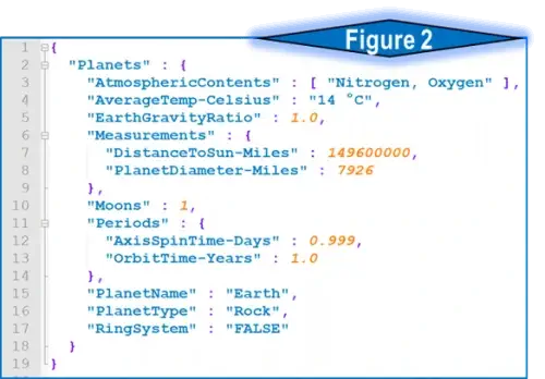
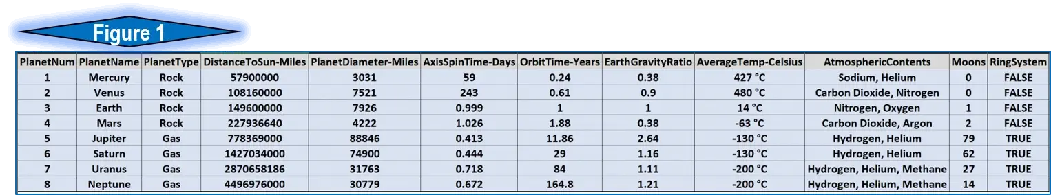
I was recently faced with the challenge of converting standard row & column table data into a very specific JSON format. The table in figure 1 is the complete data used for this example. The desired JSON formatting (figure 2) contains multiple data types, including strings, numbers, one Boolean, one array, and two embedded objects. The Table to JSON KNIME node is likely the correct approach, but the complex and indented nature of this JSON requires a unique procedure for our workflow. The various node options are detailed below.
Workflow Approach
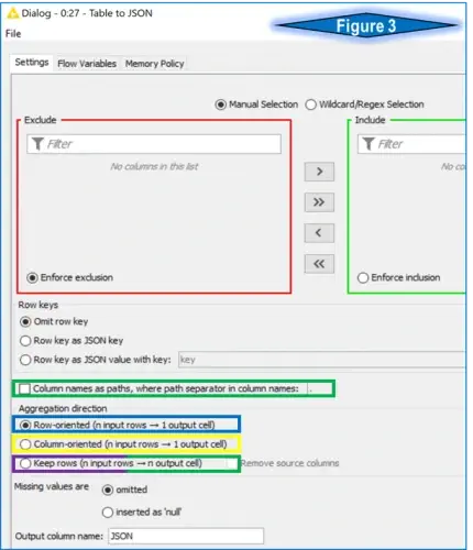
The initial concept for a KNIME workflow is to read in CSV data, permute or transform the data and output as a formatted JSON file. As mentioned above, the Table to JSON node will do the heavy lifting. Examining the node’s configuration reveals multiple options, as seen in figure 3.
The Table to JSON configuration menu has several tuning options to meet the desired output. The commonly seen Exclude/Include boxes let you choose the columns intended for output as JSON. For this example, I use the default setting of all columns.
The Row Key options allow for enumerating or tagging each JSON object with a unique identifier. This option is not required for this exercise.
The Aggregation Direction options are the key features used to convert regular table data into JSON format. The following images and explanations are color-coded to the outlined features in figure 3 (note: the purple & green feature is used twice). For reference, the data used is represented in figure 1 above.
The Row-Oriented Aggregation
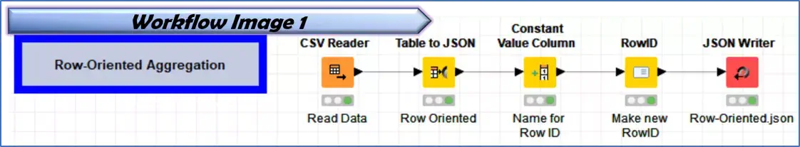
Workflow Image 1 shows a process that reads the CSV data and uses the blue-outlined aggregation in the Table to JSON process before creating a row ID and outputting the file. This process outputs one file with all the data.
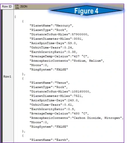
The row-oriented aggregation will convert the CSV table data into an array of JSON objects with each table row formatted as one object (see figure 4). This default configuration is simple to use and produces a somewhat expected result – our table data formatted into a simple JSON. When comparing the output from figure 4 against the intended goal represented in figure 2, the differences are apparent. The row-oriented output places all the data into JSON objects as key-value pairs, at the same indent level, rather than the more complex, embedded target JSON format. If an array of simple JSON objects were the desired output, the default configuration would be a quick solution.
Column-Oriented Aggregation
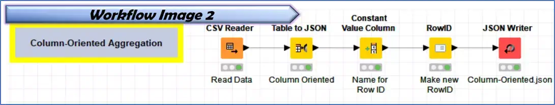
Workflow Image 2 shows a process that reads the CSV data and uses the yellow-outlined aggregation in the Table to JSON process before creating a row ID and outputting the file. This process outputs one file with all the data.
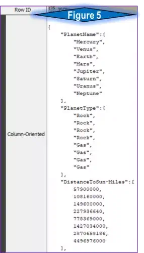
The column-oriented aggregation will compile all the data from each table column in array form and output into one JSON object (see figure 5). While nowhere near the intended output, this creates an interesting result with all attribute values within an array. A later example will demonstrate the creation of arrays within JSON objects, but with a specified target instead of the entire dimension of data.
Keep-Rows Aggregation
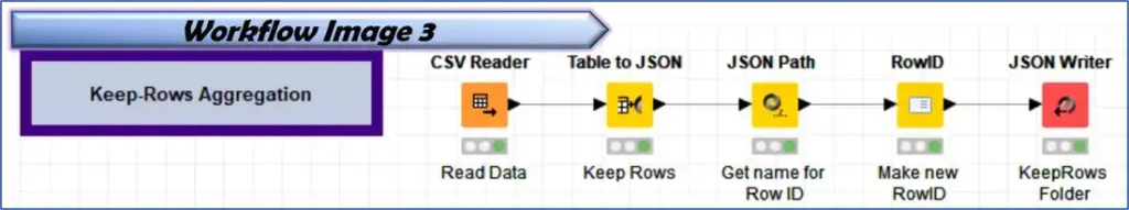
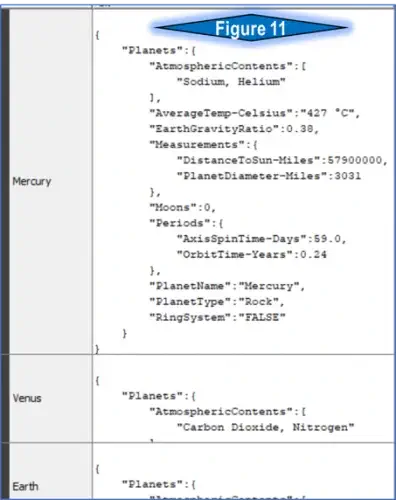
Workflow Image 3 shows a process that reads the CSV data and uses the purple/green-outlined aggregation in the Table to JSON node before creating a row ID and outputting the file. Configure the JSON Path node to query the planet name to provide a useful row ID. This process will generate an output of one file per data table row.
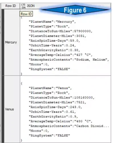
This configuration setting performs a transformation similar to the Row Aggregation above. A useful and notable exception is that now each original CSV table row feeds into a separate KNIME table row with a single JSON object. Figure 6 shows the subtle differences between this and Row-Oriented.
Keep Rows – Columns as Paths
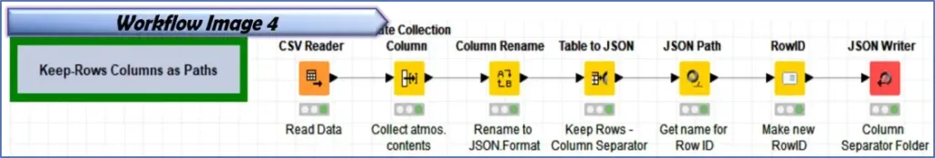
Workflow Image 4 shows a process that reads the CSV data and uses the purple/green-outlined aggregation in the Table to JSON process. This process will provide the most control over the JSON output and the final example. The following steps will describe each node, its configuration, and output.
Step 1: The Read CSV node converts the CSV file in figure 1 into a KNIME data table.
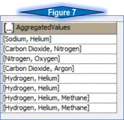
Step 2: The Create Collection Column node is used to combine the atmospheric contents column into an array column, which will remain in array form inside the JSON object. Select the multi-value column, “AtmosphericContents,” in this case, and elect to remove the aggregated column. See figure 7 for the expected output.
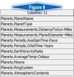
Step 3: The Column Rename node is vital to this process due to the nature of the desired output. The intended JSON is an object named “Planets” with several name/value pairs, including an array of “atmospheric contents” (square brackets [ ] ), and objects inside “measurements” and “periods” (curly brackets { } ). A closer look at figure 8 shows how this was possible. The column renaming follows a critical theme. All columns are renamed starting with “Planets.”, followed by the name of the JSON name/value pair. In the instance of embedded objects (measurements and periods), notice the renaming goes one step further to “Planets. Measurements” and “Planets. Periods” followed by the name.
Step 4: The Table to JSON node only has three aggregation settings, so this final process will utilize the ‘Column names as paths’ option, which is toggled on with a period as the separator (see figure 9). The super-power of this node works wonderfully with the newly renamed columns to provide a high level of control over the JSON object.
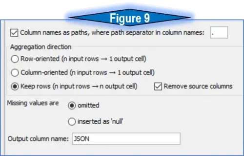
As discussed in step 3, each name/value pair is inside the Planet object JSON. When a syntax of name/name/value is employed, the data has essentially indented a level inside of a new object (Measurement or Periods). The Table to JSON places the name/value pairs for measurements (for example) into comma-delimited pairs within the measurement object.
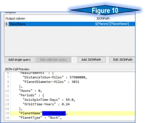
Step 5: The JSON Path node is a simple way to query within a JSON object, and will allow us to query out the Planet name into a new column. Inside the node configuration, click on the value of the desired name/value pair and press the ‘Add Single Query’ button. The name of this column will be used in the next step. Notice the dark blue box in figure 10, covering the desired value of the planet name/value.
Step 6: The Row ID node will take a specified column and replaces the row name with the value in that column. The queried value from the last step, planet name, becomes the new row name (and future file name)