Making the Pass, Part 2: Training a Neural Network with KNIME
In my previous blog posting, I started to explore what it would take to teach a machine learning model how to throw a virtual football to a moving target. If you have not read that article, please go do so: it covers the definition of the problem we are trying to model and how I used KNIME’s parameter optimization nodes to generate the parameters for completing a pass for an arbitrary set of starting conditions.
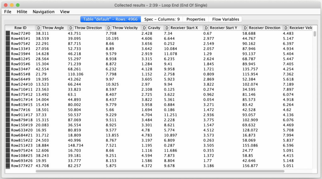
Now that we have figured out how to make a single pass give a set of starting conditions, the first step for this posting was to generate a sufficiently large set of completed passes that we could train and evaluate a model with. To do this, I simply copied the single pass generation workflow nodes into a new workflow and used several instances of KNIME’s Random Number Assigner nodes to create random starting conditions for 5,000 passes and had the single pass solver generate the pass parameters for each of them.
I am not going to go into the details of the data generation workflow; if you would like to explore it, you may download it from the KNIME hub. Since it takes several hours to run, I have used it to generate a sample data file which is already bundled with the neural network training workflow. One interesting thing to note is that even though I started with 5000 passes, I discovered that certain combinations of my starting parameters resulted in situations where my single pass parameter generation could not find any way to make a completed pass. This resulted in the final training set consisting of only 4,966 records.
With a freshly generated set of training data in hand, I then started to build a new workflow for training a machine learning model. This training workflow may also be downloaded from the KNIME hub.
As I started on the workflow, the question that immediately arose was “which machine learning algorithm to use?” Since the throw parameters are numerical, I was looking for regression models and not categorical ones. But I also had given myself the challenge of trying to solve for three inter-related parameters: the throw direction, the throw angle, and the throw velocity. This is known as multi-target regression. Since many of the most common algorithms only support the prediction of a single regression parameter, I could either experiment with trying to combine three separate single-target regression algorithms or look for an algorithm that supported multi-target regression. Based on my experience and intuition, I went with the latter approach: the task of predicting multiple numerical outputs made my problem a natural fit for a neural network.
Furthermore, I decided to use the Keras deep learning library with a TensorFlow back end. This choice was based on the fact that KNIME provides extremely flexible Keras nodes that make it very easy to experiment with various neural network configurations. Keras is implemented in Python but KNIME supports seamless integration with Python so you do not need to be a Python programmer to use it. You will just need to install a Python environment and point your Knime installation at it (a process that is well documented by KNIME).
The first stage of the training workflow is to prepare the training data. This consists of reading the source training data, normalizing it (a standard practice for neural networks), and then partitioning it into a training set and a validation set. When normalizing data for training a machine learning algorithm, one common mistake is to not save the model used for normalization. The normalization model used for training an algorithm must also be the one used when processing new data with the trained model or the predictions will be inaccurate if the input domains differ in any way.
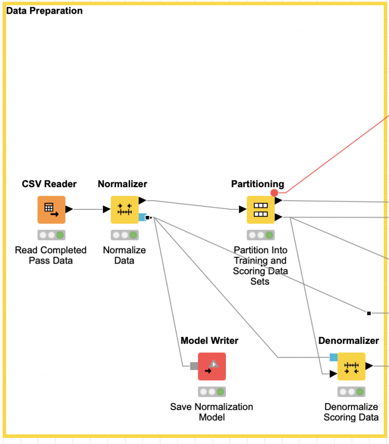
By partitioning the data into training and validation sets up front, we will have a consistent data set to use to benchmark the performance of different neural network configurations against each other. Before I started to experiment with different configuration the network, I needed to come up with a way to score their performance. Since the goal of my exercise was to teach my laptop how to throw a completed pass, I decided to count the number of completed passes each trained model made for the set of training data. The model that completed the most passes would be the best one to use for our simulation.
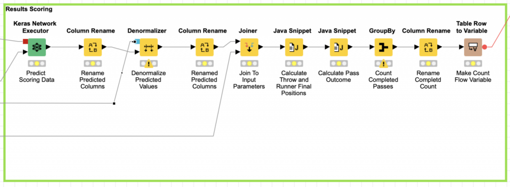
To calculate this score, I am using KNIME’s Keras Network Executor node to apply a network model to the set of validation data. For each record in the data set, I use the resulting predicted throw parameters to calculate where the pass will land and the position of the receiver at the time the pass lands. It is then trivial to calculate the distance between the ball’s landing location and the receiver. This is the numerical measure we sought to minimize during our data generation phase, but I am not going to use it directly for scoring the networks.
When I defined the challenge in part one, I arbitrarily decided that any pass that arrives within one unit of the receiver is considered a completion. For scoring the validation data we categorize each pass as complete or incomplete based on whether or not it landed close enough to the receiver. Thus, the count of all completed passes in the validation data set is the measure used to score each network’s performance with the goal being to maximize this value.
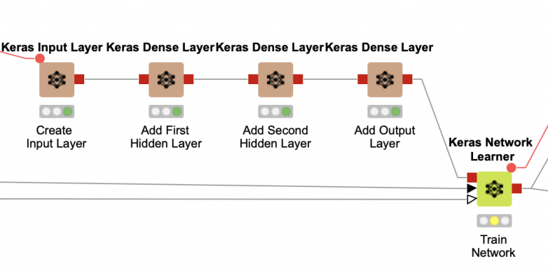
Now that we have our data preparation stage and a scoring stage, all that is left is to figure out the middle stage: configuring and training the neural network. For the network configuration, we know that the input layer of the network is determined based on the training data; we will use 5 input nodes that correspond to the initial play data (receiver start X, receiver start Y, receiver direction, receiver velocity, and gravity). Similarly, the output layer is fixed to three nodes which correspond to the pass parameters (throw direction, throw angle, and throw velocity).
At this point, I just needed to decide how many hidden layers to use and how big each of them should be. Based on my experience with Keras, I suspected that a single hidden layer would not be enough, and I tried a few initial experiments with single hidden layer networks of various sizes to confirm this. After these initial tests, I settled on using a network with two dense hidden layers (in a dense layer, each node is connected to all of the others).
In order to determine the optimal size for these two layers, I again turned to KNIME’s parameter optimization nodes. I configured the Parameter Optimization Loop Start node to try combinations of node count from 5 to 30 for each layer (a total of 676 possible combinations). The Parameter Optimization Loop end node was configured to seek the maximum possible value for the completed pass count from our model scoring stage. I did not select any parameter search optimization; I wanted to use the brute force approach to try every possible combination because I thought it would be interesting to see visualize the results to see if there were any discernible patterns in accuracy based on network size (the darker the square, the more accurate):
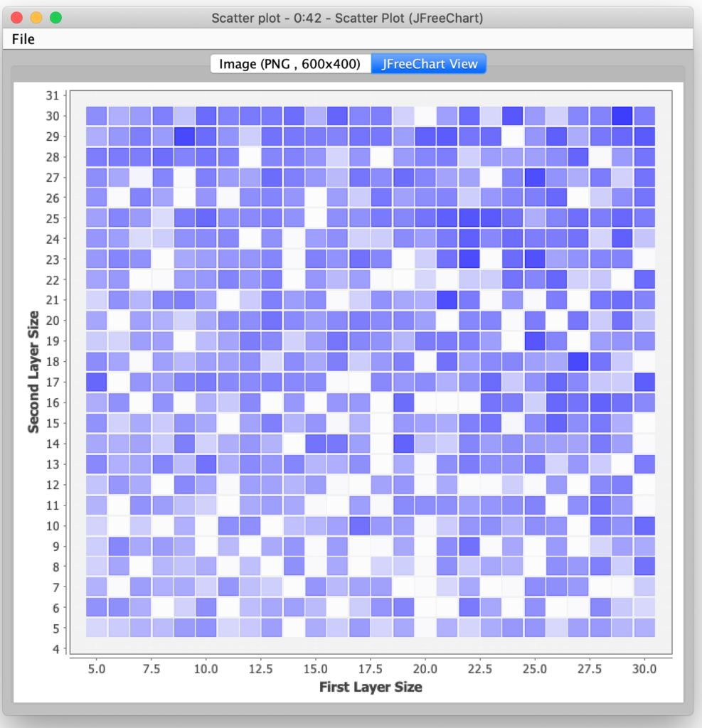
In the end, the most accurate neural network had 29 nodes in the first hidden layer and 30 nodes in the second hidden layer. I was a bit surprised that so many nodes were required for the most accurate network. For the sake of expediency, I decided not to try and explore even larger networks since I was just doing this exercise for a blog posting and not for use in a production system.
Armed with my best performing neural network, the final step was to examine the overall performance of the network on a fresh set of pass data. To do this, I reconfigured the data generation network to produce a new set of 1000 records that were produced with different randomization seeds (so that I was not simply regenerating the same records that were in the training set).
To benchmark the network, I created a third and final KNIME workflow that can also be found on the KNIME hub. The workflow is bundled with the data normalization model, the Keras neural network model, and a test data set so that it can be run independently without having to first run the data generation or training workflows.
This final workflow is straightforward: it reads the data and models and then evaluates the network against the fresh set of play data and categorizes each record’s prediction as complete or incomplete. When I ran this workflow for the first time, I was disappointed to discover that my most accurate network still had a 41.8% completion rate. Based on this, I added several scoring and visualization nodes to help me characterize the results to see if I could determine why my machine learning quarterback was throwing so many incomplete passes.
Since the scoring measure of distances from the ball is calculated from the three predicted parameters, I first decided to examine the accuracy of the individual parameter predictions by using the KNIME Numeric Scorer node to calculate various statistics between the actual values (as generated by the first workflow) and the predicted values.
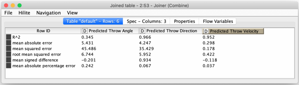
These numbers showed that the model was producing very accurate predictions for the throw direction and throw velocity, but the throw angle predictions were much more error prone. Since the parameters all interdependent, it could be that the throw angle was being adjusted the most to make up for the variances in the other two parameters (e.g. if you throw a ball at a shallower angle, you will need to throw it faster to increase its distance). Perhaps the results could be improved by predicting throw direction and throw velocity first, and then use those predictions as inputs (along with the initial data) to another model that just predicts the throw angle?
This made me wonder if I could better characterize the failures: maybe the model falls apart for longer passes? To visualize this, I plotted where the 1,000 predicted throws landed and colored the plotted by their accuracy:
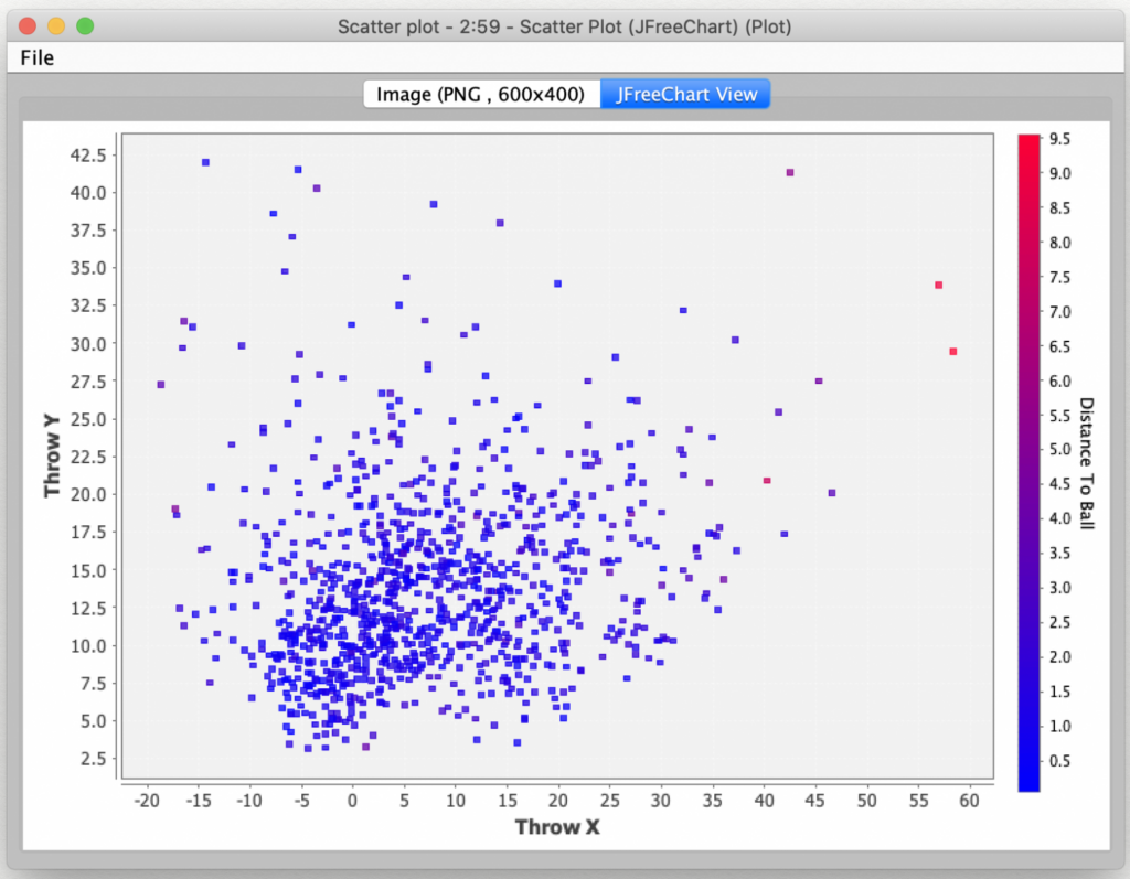
This did seem to show that the farthest outlying throws definitely had some of the worst accuracy. But what really struck me was how many throws seemed to very close (the blue colored ones). So, I decided to look at the throws’ distribution by their distance from the receiver. To do this, I assigned each throw to a bucket based on the number of units away it landed (0 to 1, 1 to 2, etc.) I chose this interval because the first bucket would represent all throws that were considered to be caught (and contributed to the score that was used for algorithm selection).
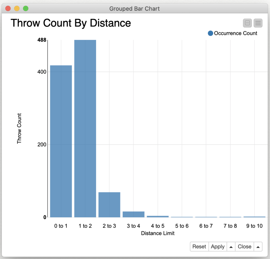
The results were surprising: 90.6% of the throws arrived within two units of the moving receiver and 97.5% of them arrived within three units. By using KNIME’s powerful histogram visualization node, we can interactively explore the nature of the distance error:
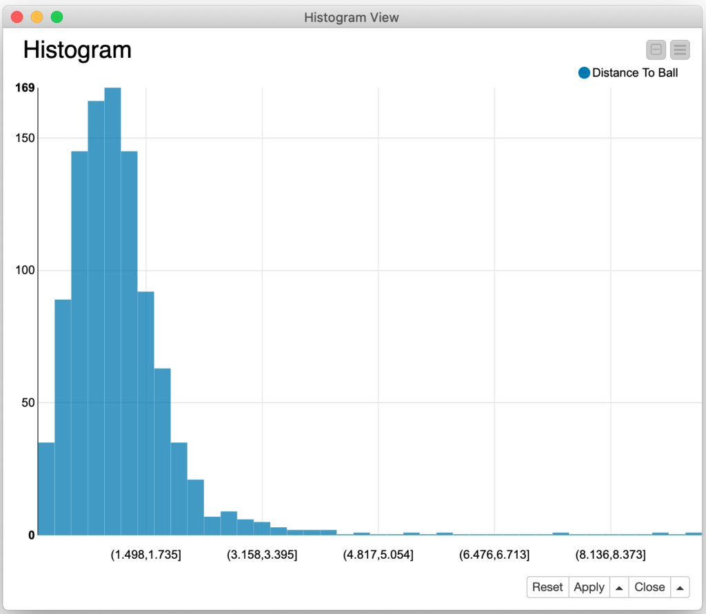
When looking at the numbers, it is much clearer that the model is doing quite a good job of predicting throw parameters that get the ball relatively close to the moving target. When I set up my problem model, I arbitrary selected that only throws that arrive in one unit would be considered to be completed. Had I selected a larger value in part one of this exercise, I’d be reporting much more successful results. This is the danger of imposing an arbitrary classification on my modelling; could I have come up with a better model if I had modelled the distance from the receiver in a more numerical fashion? For example, I could have designed a “likelihood to be caught” function based on the inverse of the distance of the throw from the receiver. If the goal of the model training was to maximize this likelihood, perhaps I would have achieved better results?
So, did I succeed in what I set out to do? Did a teach my laptop to throw a pass to a receiver in motion? Based on the average distance error, I believe I did. However, at a 41.8% completion rate, it is definitely not a professional quarterback (Drew Brees led the professional football league in 2019 with a 74.3% completion rate.) But more importantly, I hope I was able to bring you along on the process involved to define a problem and then train and evaluate a machine learning model to attempt to solve it.
In addition, I hope this pair of blog postings also show you just how nimble the open source KNIME platform can make you when are exploring data and building models. I encourage you to experiment with these workflows and I would love to hear from anyone who trains a better quarterback than I did!