What the Farkle? Recursion, Modeling, and Genetic Algorithms with KNIME, Part 3
In my previous two blog postings in this series, I’ve covered the basics of the dice game Farkle and developed a simple way of modeling player behavior so that I can attempt to evolve an optimized playing strategy using a genetic algorithm. Now it is time to finally get into how to actually implement this evolution in KNIME, a powerful open source data science platform.
In programming, a genetic algorithm is a search algorithm to efficiently find an answer to problem that does not lend itself to an exhaustive analysis. A genetic algorithm uses the notions of Charles Darwin’s theory of evolution in five phases:
- Initial population
- Fitness function
- Selection
- Crossover
- Mutation
Each generation of evolution is performed by repeating these steps using the output from the previous generation as the initial population for the next iteration. The initial population for the first generation is independently generated with goal of producing a diverse starting population so that there is a good chance most optimal traits are represented. I covered how I generated the initial population for this experiment in part two. You don’t need to run that workflow: I’ve taken its output and embedded it in my evolution workflow which you may download from the KNIME hub.
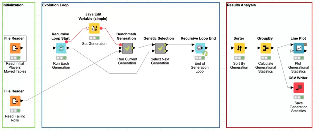
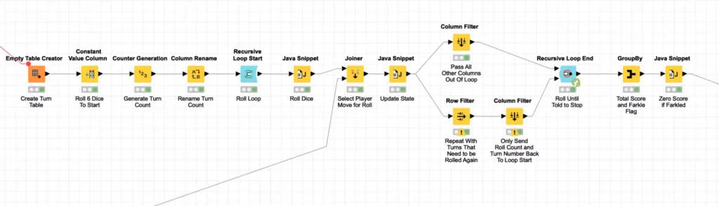
Upon initial inspection, this workflow is deceptively straight forward and you can map the 5 evolution phases onto the various processing nodes in the workflow. This is thanks to one of my favorite features of KNIME: you can nest workflow processing steps in meta-nodes. In this case, the Run Current Generation and Select Next Generation nodes in the workflow are meta-nodes that abstract away the actually processing steps and make it easy to follow the conceptual processing flow without getting lost in the details.
These nodes are surrounded by two other simple to use but incredibly powerful nodes known as the Recursive Loop nodes. These nodes work together to enable you to use the output from one loop iteration as the input to the next iteration. The Recursive Loop Start node simply takes its input and passes it in as the data for the first iteration of the loop. In our case, this is the initial player model data that was externally generated. The data is run through the other phases of the genetic algorithm and the results are sent to the Recursive Loop End node.
But if you look at the workflow above, you’ll notice that there are two inputs to the Recursive Loop End node. The first input works just like the other more traditional loop nodes in KNIME, its data is collected for the loop output. Which means that the second input is for the data that should be sent back to the loop start to be processed for the next iteration. This will be repeated an arbitrary number of times until a stopping point is reached. In the mathematical definition of recursion, this stopping point is known as the “base case.”
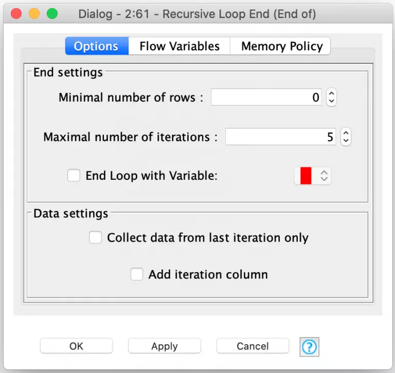
And the true power of this pair of nodes comes from the flexibility with which KNIME allows you to configure the conditions that will end the recursive loop. There are three different conditions which can be configured. The first is the minimal number of rows: the loop can end when there are not enough rows in the second input to continue processing. Since I am running a set number of generations for my player evolution, I’ve set this to zero so that there are always enough rows to continue processing. I then use the second configuration option to set a fixed number of iterations for the loop (5 in this example).
The third and final condition is to have the loop’s termination controlled by a flow variable. With this option, you can implement any conditional logic you want in a snippet node and set the flow variable appropriately. This is extremely powerful and can be used for more than just data processing. For example, you could use it to build a retry loop that continuously samples an external data source for information until a certain condition is met.
Now that we’ve looked at the main evolutionary loop, let’s look inside how we score each player in a generation. This is done with a Monte Carlo simulation that plays 5,000 turns for each player and then calculates their average score. This is done inside the Benchmark Generation meta-node as follows:
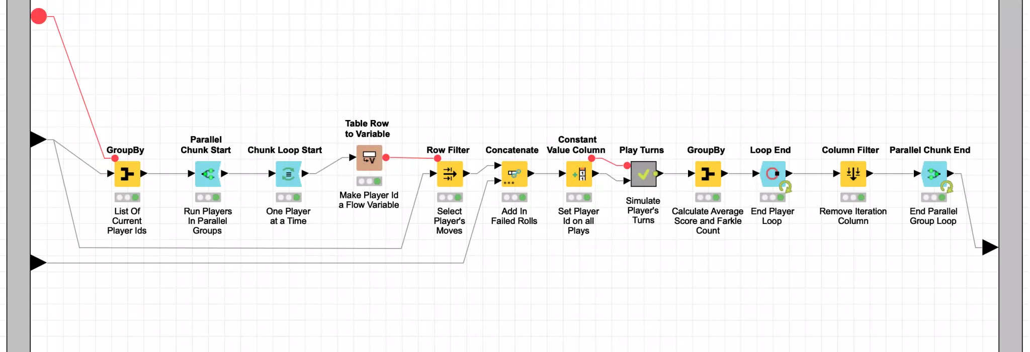
Because each player is scored independently of the others, I can leverage another powerful set of KNIME nodes to improve my workflow’s performance. These are the Parallel Chunk nodes and they are used to split up data into similarly sized chunks that can be processed concurrently to maximize the use of available CPU resources. KNIME is even smart enough to set the chunk count based on your available processors or you can specify your own custom chunk count if you want to more explicitly control resource usage.
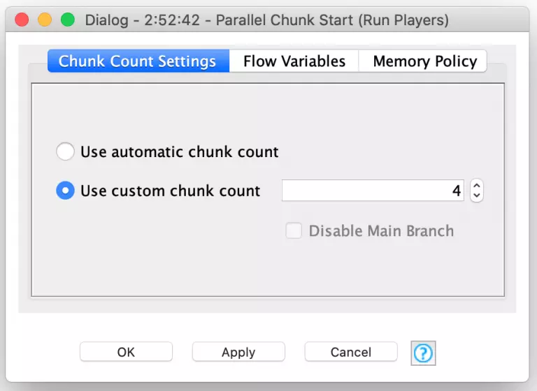
In my benchmarking section of the evolution workflow, I split up the 400 players in a given generation into four chunks of 100 players each. Each of these chunks is processed in parallel but inside each chunk, the 100 players are processed sequentially. Each player’s move table is used to play 5,000 turns inside the Play Turn meta-node. The score results of these turns are then averaged (with Farkles counting as zero points) to produce an average score for that player. Each player’s aggregate score is then fed into the Parallel Chunk loop end node which accumulates the results from all four chunks into a single consolidated data table for further downstream processing.
At this point, you may have noticed that I again used KNIME’s meta-node to encapsulate another layer of processing. The simulating of 5,000 turns for each player is a Monte Carlo simulation that is encapsulated in the Play Turns meta-node I mentioned earlier:
Because I am using a simplistic model of player behavior, each turn for a player is independent of the others which enables me to optimize this Monte Carlos simulation. Specifically, I generate all of the dice rolls at once by creating an empty table with 5,000 rows and then rolling the dice by randomly selecting an integer between 1 and 6^6. This number is then translated to a specific dice roll using the technique I discussed in the first article in this blog series.
Since any given player turn can involve re-rolling one or more dice until the player decides to stop or Farkles (e.g. does not roll any more scoring dice), the simulation needs to loop for an indeterminate number of times for all of the player’s rolls. The Recursive Loop nodes are perfect for this. In this case, we set the loop termination condition to be when there are no more turns that need another roll. This is done by setting the minimal number of rows in the Recursive Loop End configuration to 1.
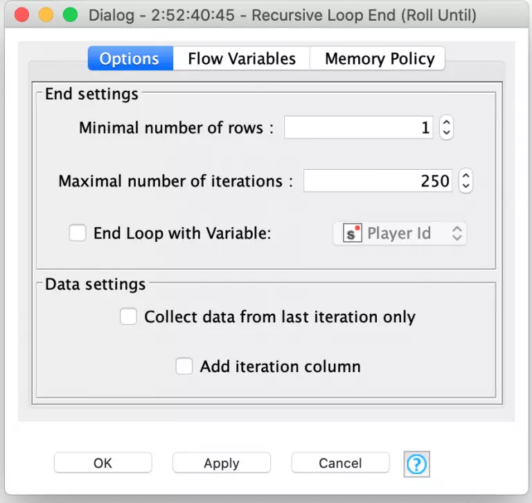
Notice that I also set the maximal number of iterations to 250. I did this as a precaution in case I had a bug inside of my loop logic for determining if the player should keep rolling. If there was a bug that caused the loop to repeat infinitely, KNIME would arbitrarily end the loop when it ran 250 iterations. The loop logic for determining if and when to reroll is done by joining each dice roll to its corresponding roll in the individual player’s move table:
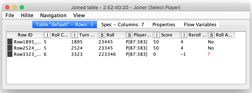
The player move table contains columns indicating the score for the current roll and how many dice should be rerolled. In this case, the first two turns (#1895 and #2524) both are scoring 50 points for the 5 and then re-rolling the other four dice. The third roll (#3323) has managed to Farkle by not rolling a single scoring di out of all six dice that were rolled. The last column in the table indicates the player’s decision of whether or not they are going to re-roll and in both of these scoring rolls, this player is going to choose not to re-roll.
The results of each roll are then evaluated in a Java Snippet node to determine if they have Farkled or if they are going to keep rolling (and how many dice they will re-roll):
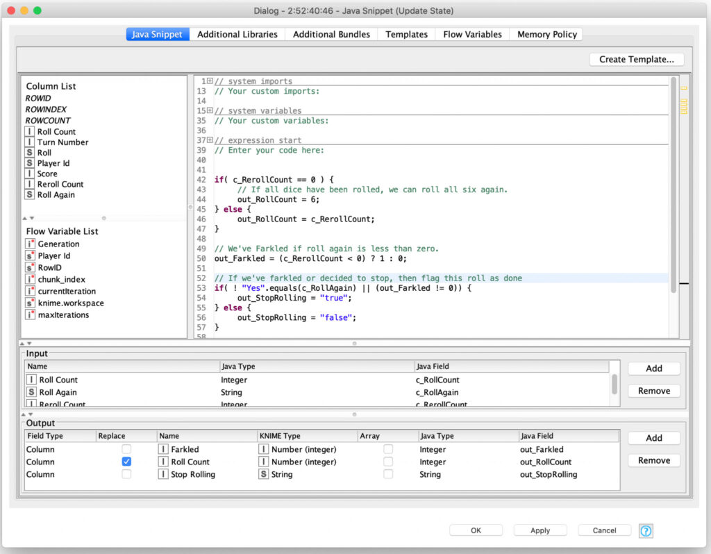
The results of this processing are filtered so that all rolls are sent out of the recursive loop but any turns that need to continue rolling dice are also sent back to the start of the recursive loop to reroll the requested number of dice. This loop continues until there are no more turns requiring further dice rolls and the loop ends.
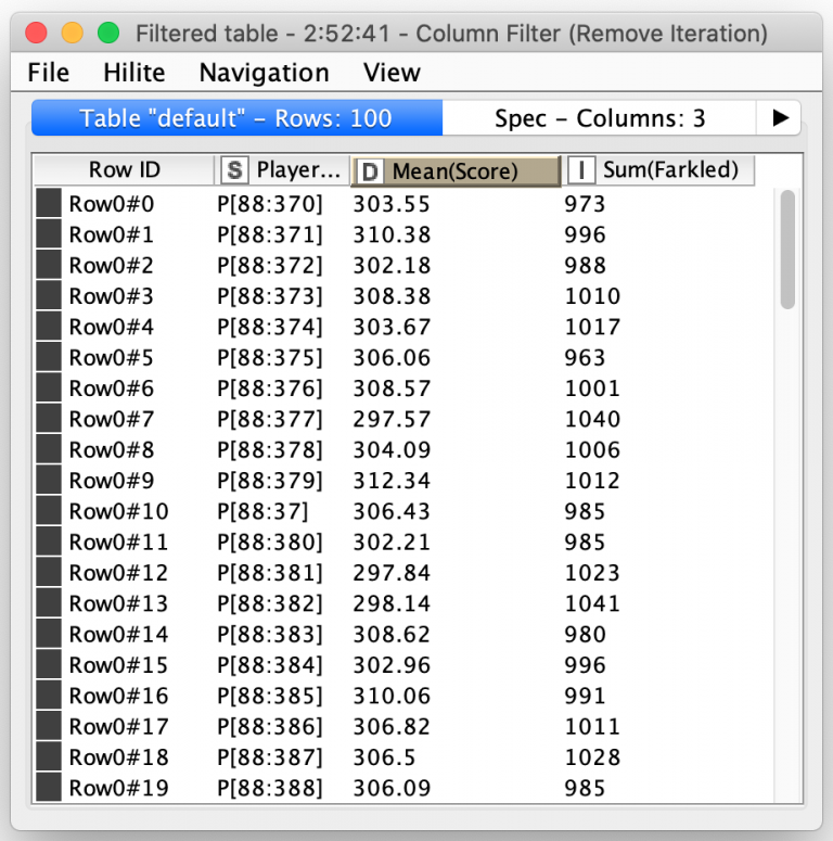
Once the simulation of all of the 5000 turns for a player is complete, each turn’s total score is calculated including setting it to zero if the player Farkled on that turn. All of the turns’ scores are then sent out of the meta-node where they are averaged to compute a single score for each player along with a count of the number of turns that player Farkled on:
From there, genetic selection of the fittest players is simply a matter of picking the ones with the best average scores. And yes, KNIME has a special node for that: The Top k Selector node. It combines the sorting of nodes and selection of the first k records after sorting:
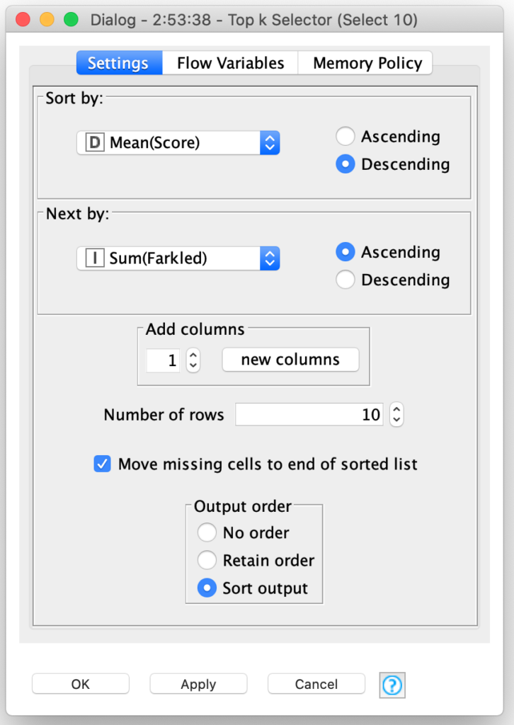
In our case, I am selecting the top 10 players from the 400 players in the generation. This was somewhat of an arbitrary choice, but I will explain my reasons for doing so when I tackle how I implemented the cross breeding and mutation phases of the genetic algorithm in my next blog posting.
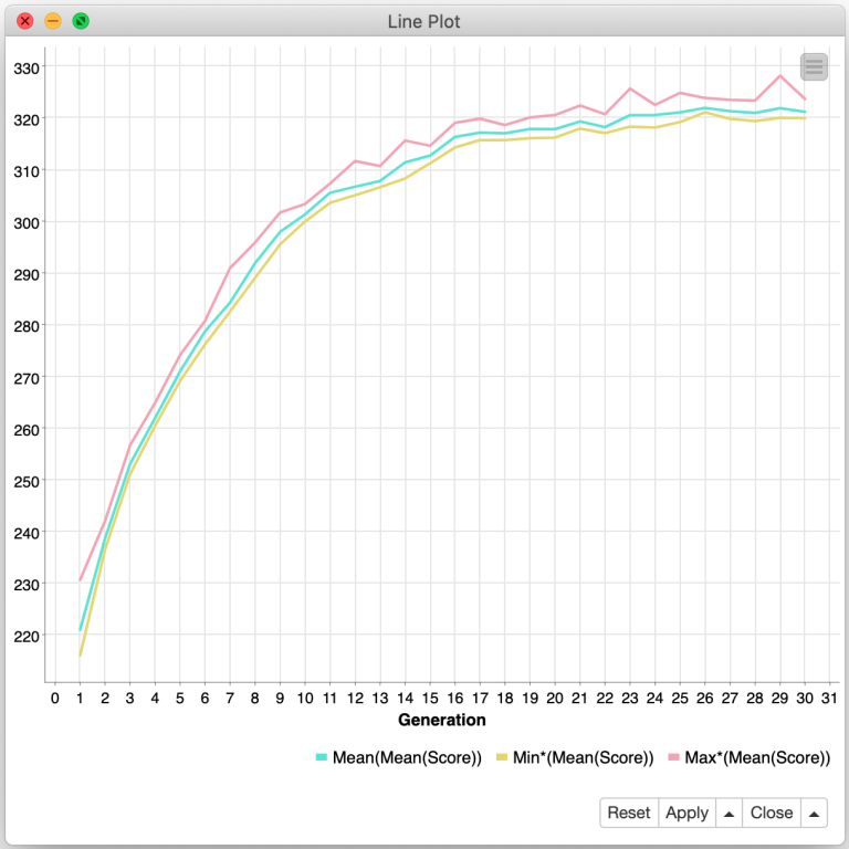
Yes, with all this processing (and my three lengthy blog entries), I have only covered the first three phases of the genetic evolution algorithm. In the fourth article in this series, I will cover how I implemented the final two evolutionary phases and do an analysis of the training results over many generations. And just maybe I will reveal the results of a head-to-head competition between my wife, myself, and the highest scoring player model that my genetic evolution algorithm produces.