Joining Fact Tables
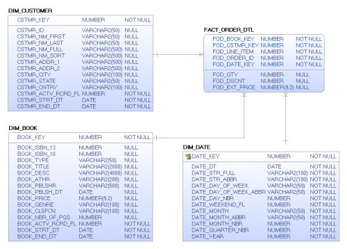
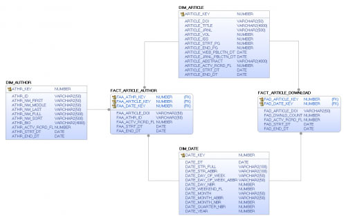
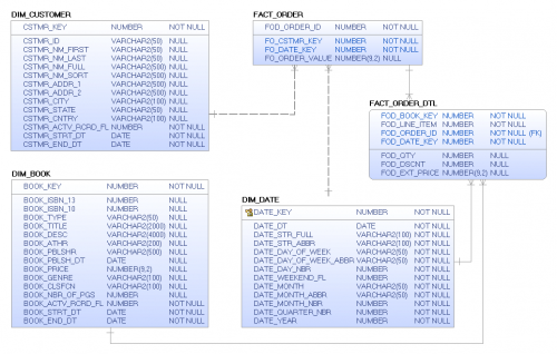
Joining fact tables can be done but there are some inherent risks so you need to be careful when joining fact tables is required. In the following simple scenario, we have a fact of authors to articles and a separate fact of articles to pageviews. Our customer has asked for the ability to 1) find the authors who have provided the most content in a given time period, find the articles which have the greatest number of pageviews for a given time period and 3) find the authors with the highest number of pageviews in a given time period. Our data model can be seen here:
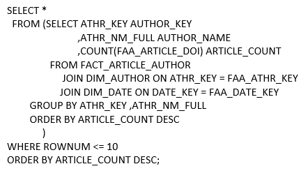
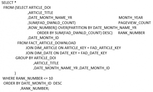
To answer the first two questions is done by using a simple select statement joining a single fact table with the date dimension and the associated other associated dimensions to retrieve the answer.
TOP 10 AUTHORS BY ARTICLE COUNT
TOP 10 ARTICLES BY MONTH
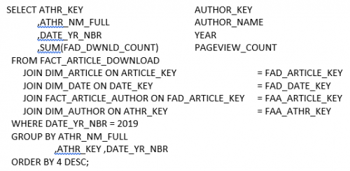
The third requirement will compel us to join two fact tables to get the answer. Remember to join a fact table you need at least one common dimension shared between the facts to accomplish this task. In this scenario, DIM_ARTICLE will be the common dimension which we will use.
TOP 10 AUTHORS FOR 2019
These simple joins work well on small and medium sized fact tables but as the fact tables increase in size your performance may suffer and therefore you may want to be prepared to address these challenges.
There are two other specific issues to be aware of and avoid, Chasm Traps and Fan Traps.
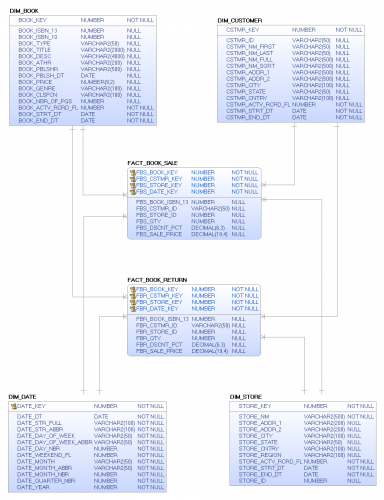
Chasm traps are queries that require measures from more than one fact table. In the data model below we see 2 separate fact tables, one for sales and one for returns. A common request may be to show the net profit (sales – returns) for the 4th quarter of 2018. We may be tempted to join these two dimensions on DIM_DATE and get the results of the sum of sales and the sum of returns.
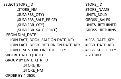
Let’s walk through the example by running each query separately. First, let’s get the total sales for each store for the 3rd quarter of 2018 using the following query:
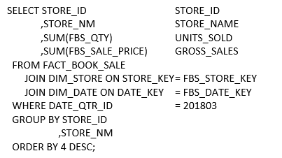
RESULTS
| Store ID | Store Name | Units Sold | Gross Sales |
| 2 | NEW YORK | 2109 | 18,532.55 |
| 7 | PORTLAND | 2094 | 18,205.14 |
| 6 | PHILADELPHIA | 2058 | 18,117.64 |
| 4 | WASHINGTON | 2062 | 17,948.92 |
| 9 | SAN FRANCISCO | 2040 | 17,647.64 |
| 5 | SEATTLE | 2034 | 17,638.31 |
| 1 | ONLINE | 2053 | 17,599.21 |
| 8 | BOSTON | 2010 | 17,286.39 |
| 3 | LOS ANGELES | 1962 | 17,008.89 |
Next, let’s get the total refunds for each store for the 3rd quarter of 2018 using the following query:
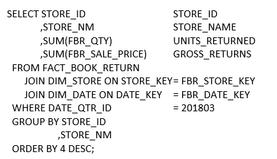
RESULTS
| Store ID | Store Name | Units Returned | Gross Returns |
| 6 | PHILADELPHIA | 68 | 602.66 |
| 3 | LOS ANGELES | 67 | 580.03 |
| 7 | PORTLAND | 64 | 569.28 |
| 2 | NEW YORK | 61 | 526.16 |
| 4 | WASHINGTON | 62 | 526.05 |
| 9 | SAN FRANCISCO | 58 | 510.32 |
| 8 | BOSTON | 52 | 442.92 |
| 1 | ONLINE | 48 | 414.57 |
| 5 | SEATTLE | 43 | 382.70 |
Finally, let’s put both of these together into a single query with the following query:
RESULTS
| Store ID |
Store Name | Units Sold |
Gross Sales |
Units Returned |
Gross Returns |
| 7 | PORTLAND | 12140 | 105,680.48 | 8007 | 69,802.46 |
| 6 | PHILADELPHIA | 11718 | 102,838.25 | 7942 | 69,391.35 |
| 2 | NEW YORK | 11692 | 101,895.82 | 7732 | 67,121.34 |
| 1 | ONLINE | 11545 | 99,375.88 | 7628 | 66,735.25 |
| 5 | SEATTLE | 11441 | 99,165.43 | 7485 | 64,984.80 |
| 4 | WASHINGTON | 11414 | 99,132.33 | 7607 | 66,445.23 |
| 9 | SAN FRANCISCO | 11434 | 99,110.30 | 7697 | 66,808.76 |
| 8 | BOSTON | 11444 | 98,324.45 | 7609 | 66,681.70 |
| 3 | LOS ANGELES | 11250 | 97,627.69 | 7442 | 64,708.52 |
The results are inflated due to the cross join which will occurs between the fact tables when trying to get a group function result.
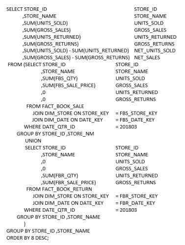
To avoid the chasm trap you need to separate the functions into the base SQL statements we originally designed to verify our results, adding zeros for the columns from the other table, and then union the statements together, wrap them in a SQL statement.
RESULTS
| Store Name | Units Sold | Gross Sales | Units Returned | Gross Returns | Net Units Sold | Net Sales |
| NEW YORK | 2109 | 18,533 | 61 | 526.16 | 2048 | 18,006 |
| PORTLAND | 2094 | 18,205 | 64 | 569.28 | 2030 | 17,636 |
| PHILADELPHIA | 2058 | 18,118 | 68 | 602.66 | 1990 | 17,515 |
| WASHINGTON | 2062 | 17,949 | 62 | 526.05 | 2000 | 17,423 |
| SEATTLE | 2034 | 17,638 | 43 | 382.70 | 1991 | 17,256 |
| ONLINE | 2053 | 17,599 | 48 | 414.57 | 2005 | 17,185 |
| SAN FRANCISCO | 2040 | 17,648 | 58 | 510.32 | 1982 | 17,137 |
| BOSTON | 2010 | 17,286 | 52 | 442.92 | 1958 | 16,843 |
| LOS ANGELES | 1962 | 17,009 | 67 | 580.03 | 1895 | 16,429 |
Fan traps occur when there is a that require measures from more than one fact table in a master detail relationship. An example of this is an order and order detail relationship.
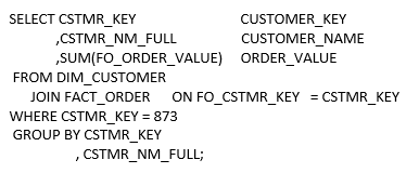
For this example, our customer has given us a requirement to calculate the average order item. If we try to sum the order value from the fact order table and then sum the quantity of items ordered from the order detail to help us get the average the order value may be inflated due to the cartesian join between the fact tables. Let’s start with a simple select between the customer dimension and the FACT_ORDER table.
RESULTS
| Customer ID | Customer Name | Order Value |
| [email protected] | Emmy Cuevas | 353.80 |
But when we add in the FACT_ORDER_DTL to the query the result changes in the sum from the FACT_ORDER table.
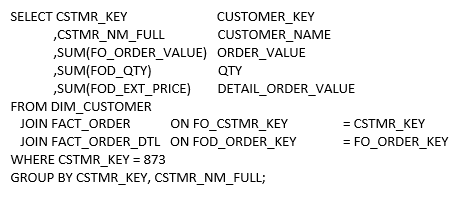
RESULTS
| Customer ID | Customer Name |
Order Value |
Qty | Detail Order Value |
| [email protected] | Emmy Cuevas | 381.70 | 38 | 353.80 |
Again, this will be exacerbated by the additional number of line items in the FACT_ORDER_DTL to the cross join between the fact tables.
The way to address this challenge can be done in multiple ways. The first is to ignore the FACT_ORDER (parent) when summing information from the FACT_ORDER_DTL (child). If you rely only on the detail table you can be assured your answer will be correct.
Another way to address this challenge is to adjust the design by removing the FACT_ORDER table and inserting the ORDER_ID as a degenerate dimensional value into the FACT_ORDER_DTL.