Making the Pass, Part 1: Parameter Optimization with KNIME

With the Super Bowl just around the corner here in the United States, I recently found myself trying to think of a football-themed blog posting.  Based on the football theme, I decided to create a post about a fundamental aspect of the game: throwing the ball to a receiver (a “pass” in American football parlance.)  It is a simple operation that, with a little bit of practice, most people can perform intuitively without any knowledge of the physics equations that govern the projectile motion of the ball and the linear motion of the receiver.  Maybe it would be possible to use machine learning to teach my laptop how to complete a pass to a moving target without just programming in the physics calculations?

Looking at this in the most simplistic manner, I want my laptop to make a bunch of random throws and learn from when they are successful. This is the essence of the class of machine learning algorithms known as “supervised learning.” The goal of supervised learning is to use training data to determine the function so well that when a new data set is given, the output can be accurately predicted.   In contrast, unsupervised learning is to model hidden patterns or underlying structure in a given data set in order to learn about the data, which does not match well with the task I’ve selected for my laptop quarterback in training.

To start the learning process, I need a set of training data but if I genuinely just used random pass data, I could generate an excessive amount of data for incomplete passes with very few positive examples of complete passes. This data would have little training value. So instead I need to come up with a training data set consisting of an appropriate number of successful passes. Note that I’m hedging here by saying an “appropriate number” as we don’t yet know what that might be – the size of the training set is likely dependent on the complexity of the problem and the machine learning algorithm that we are trying to train.

So how am I going to get this training data?  In an ideal world, I could capture completed pass data from a large number of football games, but this is way outside of the scope of a simple blog posting. Furthermore, one of my modeling assumptions that I snuck into the first paragraph of this posting was the “linear motion of a receiver.” In the real world, there are no such constraints on the motion of a receiver – they can run pre-planned routes or change their routes based on real-time conditions during the play.

Since I don’t have any easily accessible source of actual data that fits with my modeling assumptions, I’m going to have to synthesize some completed pass data for training with. My first gut instinct was just to start working out the mathematics so that I could produce a set of functions for calculating the ideal pass from a fixed thrower to a receiver on an arbitrary linear route at a constant velocity within a set of arbitrary constraints for the maximal throw velocity (e.g. no such thing as a faster than light throw).

But this felt a bit like cheating because I would both be providing mathematically perfect training data and I was also ignoring the powerful tool I had sitting at my fingertips: the KNIME Analytics Platform. What if I could use KNIME to generate some “dirtier” completed pass training data?  Did I just reason myself into a chicken or the egg problem? How can I teach my laptop to throw a football if I first must teach it to throw a football to generate training data so that I can teach it how to throw a football…? Well, it can be done, and I will walk you through the how and why – if you’d like to follow along directly in my KNIME workflow you can download it from here.

But first let us back up to the task I want to teach my laptop how to perform. Maybe if we more rigorously define it, we will find a way out of the conundrum.  So, I sketched out the problem as follows:

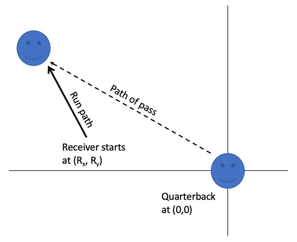
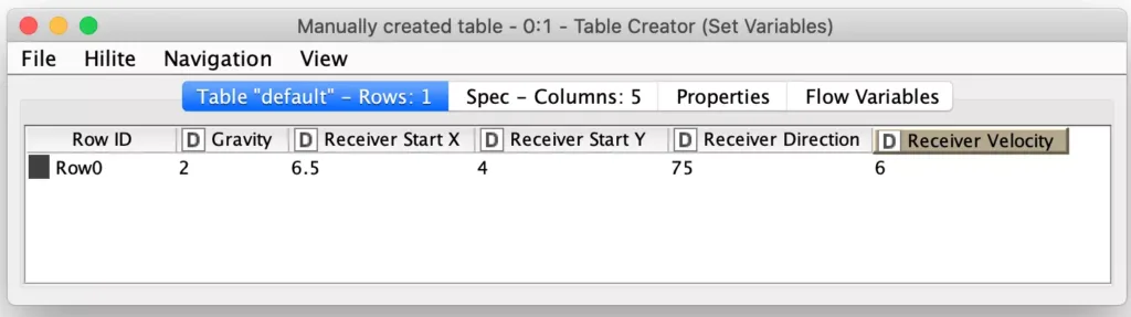
While drawing the sketch, I realized there were some arbitrary choices I could make to simplify the model. Most importantly, the quarterback would stay in a fixed position at the origin (0,0) of the coordinate system. The receiver would start at an arbitrary position Rx, Ry and run away from the quarterback in a random direction (but limited to down field) and at a constant velocity. These are what I am considering the receiver’s “run parameters.”

To make sure the pass can be completed, I will also limit the receiver’s maximum velocity to be well less than the maximum velocity of the thrown ball. I am also assuming that the quarterback throws the ball immediately (e.g. at time 0 in the model). Finally, to make the model require a little less precision, I am assuming that any throw that gets to within one unit of the receiver can be caught (e.g. there does not have to be a mathematically perfect intersection of the path of the receiver and ball and the exact time of the landing of the ball.)

There is also one other implicit parameter lurking in the model: gravity. Since the path of the receiver and the trajectory of the ball are not particularly complex in terms of their mathematics, I decided to make things a little more interesting by allowing the value of gravity to be changed for each run scenario. Thus, gravity is another initial parameter that is supplied along with the “run parameters” as the set of initial model parameters:

Based on my initial sketch, it became clear that there were only a few “things” the quarterback could do to affect the throw that they are making. They can choose the direction of the throw, the angle of the throw, and the speed of the throw.  I’m considering these the “throw parameters”.

The problem now becomes: for an arbitrary set of run parameters, what are the optimal throw parameters? To answer that question, we have to define what we mean by optimal. Obviously, an incomplete pass is not optimal but given that we have multiple throw parameters we can vary, we can make any number of completed passes. Since the goal of American football is to advance the ball as far down the field as possible, we will define optimal in this case as the pass that is caught the farthest down field from the quarterback.

As I mentioned earlier, we could just randomly pick values for these parameters until we find a set that completes a pass. This could take a long time and it would not guarantee that we found the set of parameters of that results in the optimal pass (based on our definition of optimal). But maybe we could just keep picking enough random sets of parameters until we found a large number of completed passes with the hopes that one of them will prove to be close to the optimal pass? This is BFI – Brute Force and Ignorance.   If we make an infinite number of passes, one of them is bound to be close enough to the optimal pass….

But this is not practical; particularly since we might need to generate a broad set of training data based on many different receiver’s run parameter values. What if we could guide the random parameter value selection? After all, if we make a throw in the real world, we can tell how “close” we came to hitting our target. Any miss would be considered an error, and we can even measure the magnitude of the error based on how far away the ball landed from the receiver. A person could and should learn from that error and adjust their next try accordingly.

Well, KNIME can do the same thanks to the pair of innocuous but extremely powerful nodes: the Parameter Optimization Loop nodes. These nifty nodes allow you to specify one or more parameters as flow variables and designate their range of values for each of them. The nodes will then loop over a set of nested nodes until the optimal set of parameter values is found. Sounds familiar, right? Here is the Parameter Optimization Loop Start node as configured for our data generation task:

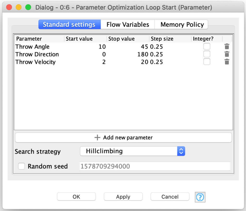
You can see the three throw parameters I discussed earlier along with the constraints on their values to fit within the model I constructed. But you may also notice that there is a configurable search strategy – this is how you tell the node the best way to find the optimal parameter sets and we cover the various strategies shortly.

As I mentioned earlier, the goal is to optimize the parameter values to minimize the error.  In our case, I’m defining the error as merely the distance between the receiver and the ball at the end of the throw and its really simple to tell KNIME to optimize that in the Parameter Optimization Loop End node:

There are two outputs from the loop end node. The first is the optimal set of parameter values (e.g. the one with the minimal error value). The second is the set of all tested parameter value combinations and their corresponding error values. This is an important distinction to make for our scenario; remember that we are not just looking for the most accurate throw but for the throw that arrives within one unit of the receiver (e.g., error less than 1.0) and results in the receiver as far down the field as possible (e.g., the maximal Y position for the receiver).

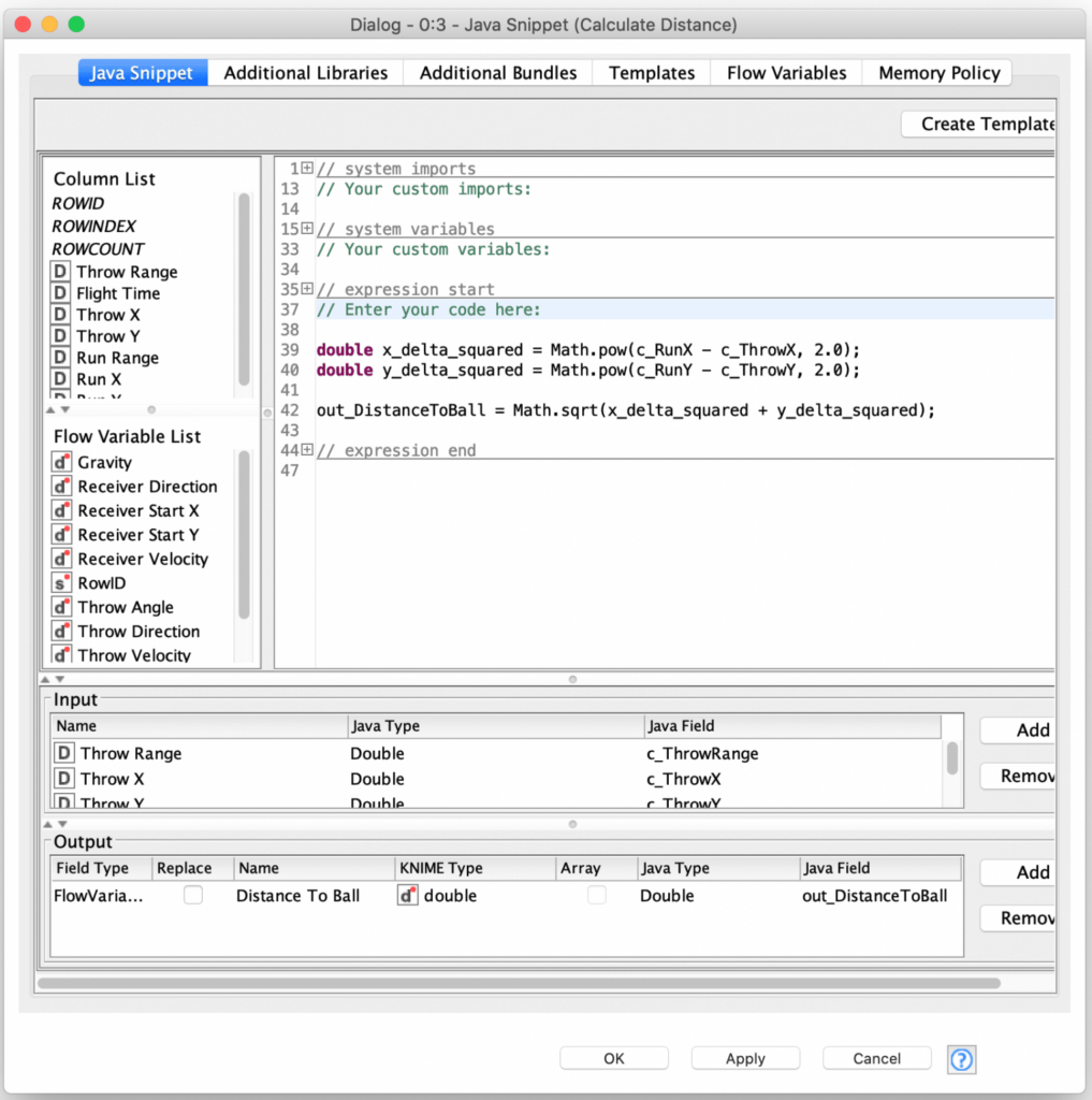
Before I go into how we select this optimal throw from the loop’s output, let us touch on what is happening inside of the loop. The first thing the loop does is calculate the throw’s characteristics based on the current set of throw parameters. This includes not just the coordinates of where the throw lands but also it’s time in flight. The time in flight is then used to calculate the receiver’s position at the end of the throw.  All of this is done in a Java Snippet node:

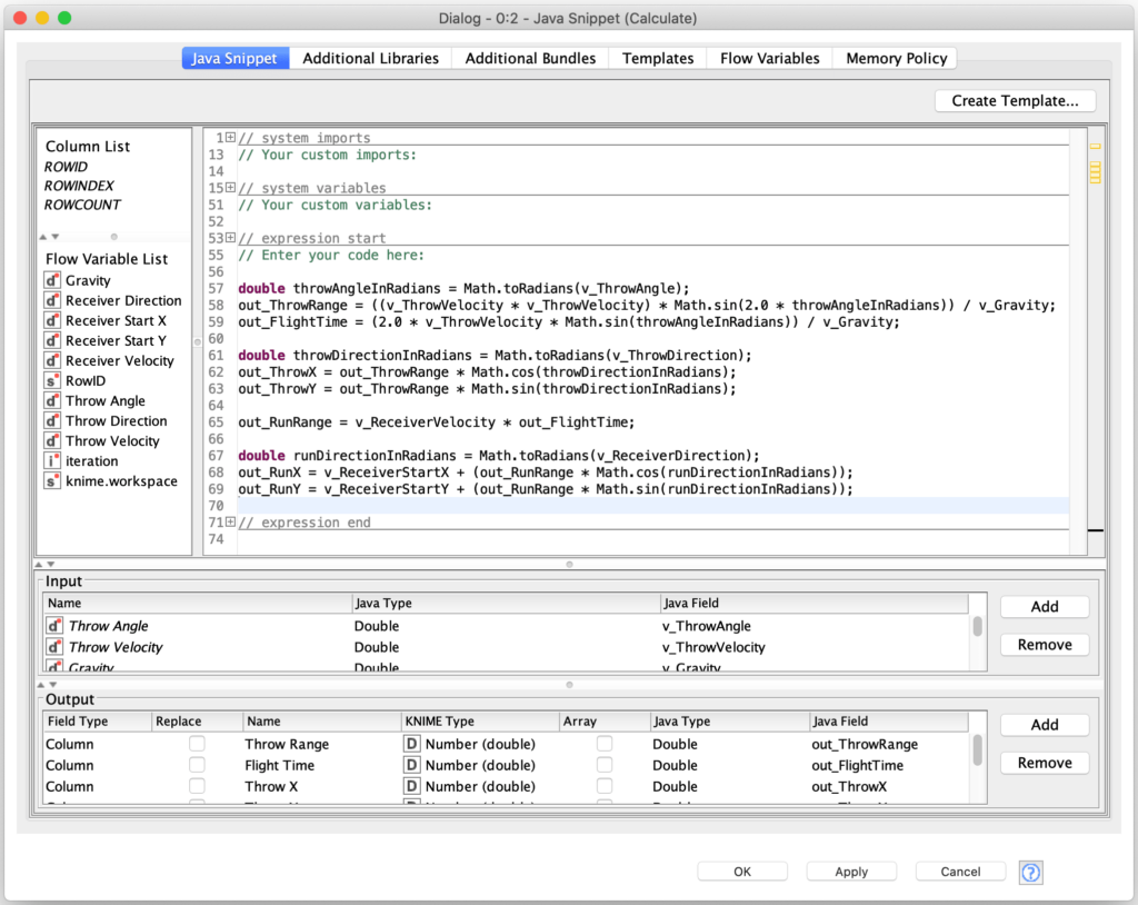
Now that we know where the ball lands and also where the receiver is when the ball lands, it is easy to calculate the distance between those two points to use as our error measure:

This is all we need to model each throw for a given set of parameters and let the KNIME optimization nodes do their magic. But I did earlier mention that the nodes support a selectable search strategy for how to search for an optimal set of parameter values. The first strategy is “Brute Force” which will try every possible combination of parameter values using the constraints and step sizes that are configured in the loop start node. If we want our data generator to finish in any reasonable amount of time this is not a practical approach for our model since it would result in many millions of iterations of the loop for each training data record.

The next impractical approach for us is the “Random Search” strategy where the loop nodes will try random values for each parameter in the hopes that one of the sets will result in a minimal error. You can tell the node how many random sets of values to try and even tell it to stop prematurely if it finds a set of values that is good enough based on a configurable tolerance. Again, with our large set of potential values and desire to find something close to the optimal throw in terms of distance down field, we need an approach that is more likely to give us the best potential sets of parameters.

This is where the remaining two search strategies come into play. The first is “Hillclimbing” where the loop picks a random starting set of parameters and then evaluates the set of all the neighbors (e.g. using the step sizes to move each parameter value in both directions) to see which neighbor moves the most towards minimizing the error. This process is repeated a configurable number of times or until no neighbors result in an improvement of the error score.

The final search strategy is “Bayesian Optimization” where multiple initial random parameter combinations are considered and then the Bayesian Optimization strategy attempts to use the error value characteristics of these combinations to select the next round of parameter value combinations to try. This also continues for a configurable number of iterations.

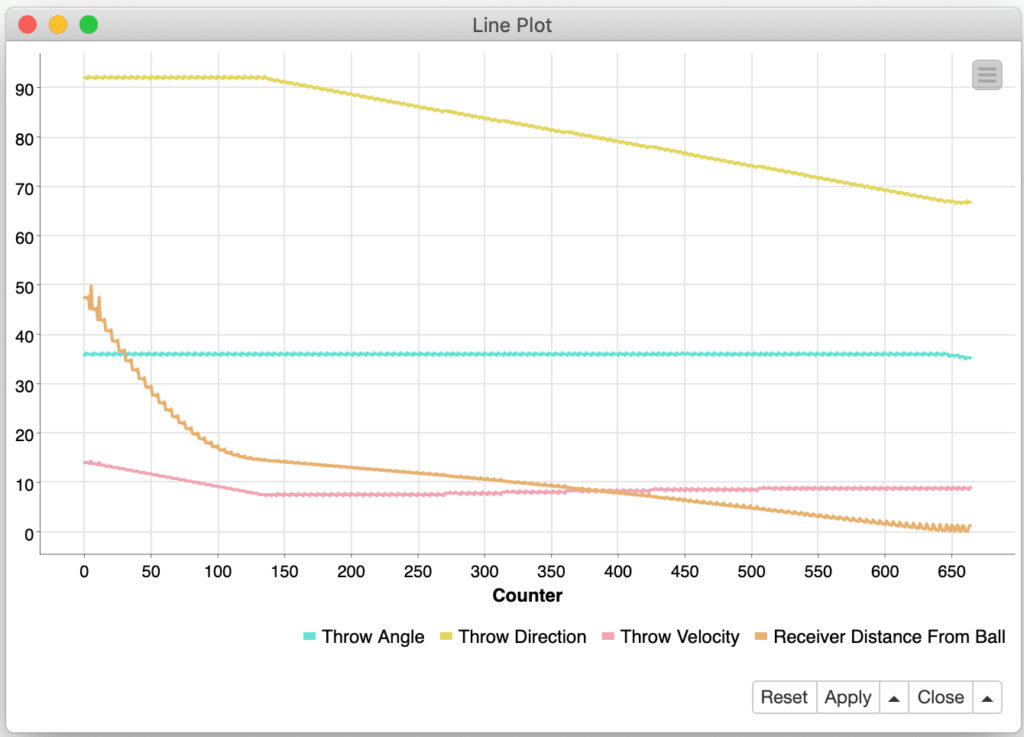
When deciding between which of the two more sophisticated search strategies to use, you need to understand the nature of your error function: how smoothly and quickly it converges and if it may have local minima instead of just one global minimum. Fortunately, you can leverage the power of KNIME to test the strategies and visualize their operation. For example, when we used the “Hillclimbing” strategy you can see the loop start with a relatively large error of almost 50 units from the ball and it initially adjusts the velocity and then soon starts adjusting the throw direction before finally tweaking the angle of the throw:

If we switch to the “Bayesian Optimization” strategy, you see a much more chaotic search since it is starting from multiple random points and considering a wider variation of parameter combinations:

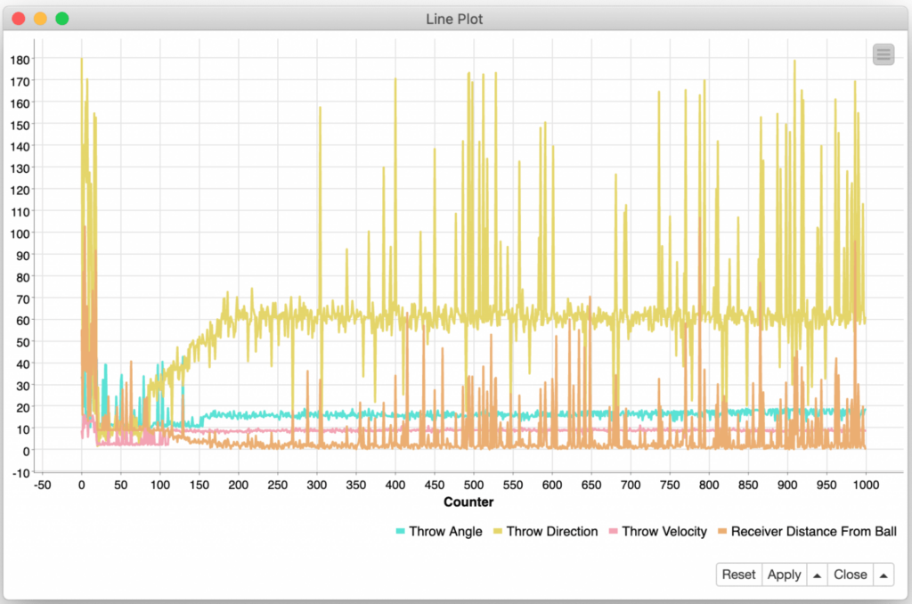
As I mentioned previously, since our error function does not optimize for the receiver’s distance down the field, we are not just looking for the lowest error score but an acceptable error score (e.g. less than 1.0 for a catch) with the largest Y distance traveled by the receiver. Based on these requirements and the above graph of the search strategy, it is clear that the “Bayesian Optimization” strategy produces many more potential completed throw candidates at the small cost a few hundred extra iterations to do so.

We then take all of the attempted parameter sets tried by the optimization loop and filter them down to just the ones that are considered to be caught (e.g. error value of less than 1.0). Since the optimization loop only outputs the parameter values and their associated error scores, we need to recalculate the coordinates of the catch and then we sort all of the completed throws based on the Y parameter of the catch so that the first record contains our optimal throw:

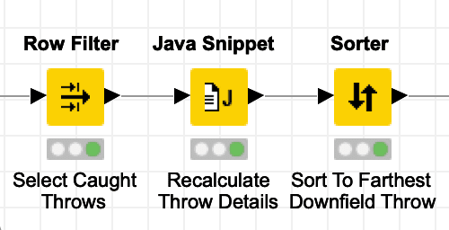
These nodes give us a table of the completed throws sorted in order from farthest downfield to least downfield:

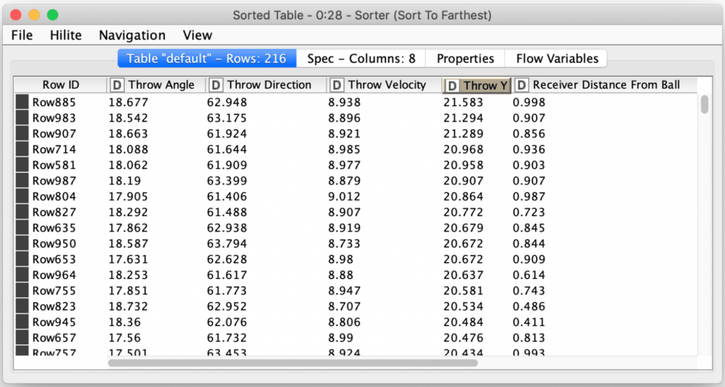
One interesting thing to note is that because we used the “Bayesian Optimization” search strategy, the best results were obtained at different iterations as can been seen from their row ID’s which were generated during the parameter optimization loop before the table was sorted on the Throw Y column.

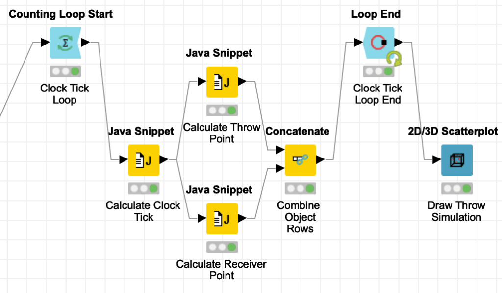
Finally, to help visualize the results and verify that the selected throw parameters are indeed accurate I’ve included a second loop that simulates the trajectory of the ball and the position of the receiver for 100 “clock ticks” evenly distributed over the flight time of the ball:

By using the powerful 2D/3D Scatterplot node, which is freely available as a KNIME community node, we can then display the simulation results in an interactive graph visualization:

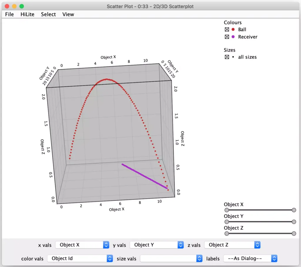
In the screenshot above, the quarterback is located at position (0, 0) in the back left of the cube. The receiver’s path is represented by the purple points coming towards the camera and angling away from the quarterback. The quarterback’s throw’s trajectory is shown by the red dots and even includes the trajectory to better illustrate the relationship between the pass and the receiver over time.

Now that we have verified that given a single set of starting receiver “run parameters” we can produce a near-optimal throw for passing to the receiver, we now need to build an enclosing loop to an arbitrary number of records with initial “run parameters” and calculate their throw parameters using the technique we evolved in this blog posting. This will be our training data set for trying to teach my laptop how to throw the ball, and my next blog posting will pick up here and cover the teaching of various machine learning algorithms and include a contest to see which one “learns the best” for our simplistic scenario.

Until then, please feel free to experiment with the single throw workflow from this blog. There are many exciting aspects to explore. For example, can you replicate the optimization loop and have two different strategies/configuration duel against each other by seeing which one completes a pass before the other? You could even wrap the current parameter optimization loop in another loop to try and optimization the configuration of the step size for the existing parameter loop. Also, if you don’t feel like playing with the workflow, you should familiarize yourself with the Parameter Optimization Loop nodes and keep an eye out for your own data analysis challenges where they can help make an impact.   In my opinion, these nodes are one of many great examples of how easy KNIME makes applying so many sophisticated data analysis techniques.