Baking an Approximate Pi with KNIME Using a Monte Carlo Recipe

With the holiday season in the United States rapidly approaching, I thought I’d have some fun with this blog posting. So rather than giving you a typical blog entry highlighting some specific cool pieces of the awesome open-source KNIME end to end data science platform, today I am going to teach you how to bake an Approximate Pi with KNIME using a Monte Carlo recipe. And along the way I will show you some interesting cooking tools and techniques to add to your KNIME kitchen.

What is an Approximate Pi you ask? It is simply an estimate of the irrational value of pi, the ratio of a circle’s circumference to its diameter. And our Monte Carlo recipe? Roughly speaking, Monte Carlo methods are a broad class of computational algorithms that use random sampling to obtain numerical results. So, in the style of the Muppets’ Swedish Chef, we are going to start cooking randomly and by doing so enough times, we will eventually bake a decent Approximate Pi.

Ok, so I’m fudging a little bit in the interest of being dramatic. We won’t be totally random; we do have a recipe after all. The Monte Carlo recipe for baking an Approximate Pi involves randomly generating sample points inside of a square (our baking sheet) and then counting which ones fall inside the largest circle (our pie tin) that fits inside the square. Given that the diameter of the circle is the same as the width of the square, through the magic of math we can determine that the ratio of the area of circle to the area of the square is pi /4. In other words, pi is approximately 4 * (the number of sample points in the circle/the total number of sample points).

Note that I am being careful to not use the term calculating in our recipe; we are estimating the value using a sufficiently large number of random samples so that our estimate converges towards the actual value. This is the power of a Monte Carlo recipe – they can be used for estimating values where doing actual calculations are impractical (such as complex odds calculations.)

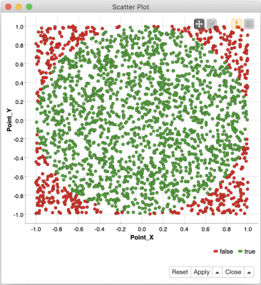
If you would like to dive deeper into the math behind this recipe, please see this nifty online demo that animates our baking process. For a quick visual example, here is an image from KNIME’s Scatter Plot node that shows an Approximate Pi we baked using 2,500 random points. The green points are in the Approximate Pi and red points sadly ended up on the baking sheet.

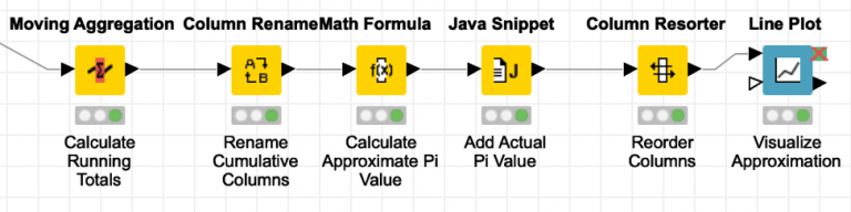
So how do we bake this recipe using KNIME as the oven? By using a KNIME workflow to generate the sample points, classify them as to whether or not they are in the circle, and count the ones that are in the circle to use in the approximation’s formula that we figured out earlier. I’ve written this workflow and made it available here for you to download and experiment with while following along.

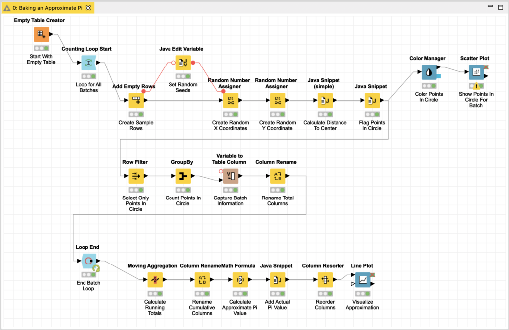
Our simple Monte Carlo recipe is an iterative process and could be done in a single loop under the assumption that the more iterations we do of the loop, the more accurate our estimate is likely to be. But since this means processing millions of points, it makes it harder to visualize the convergence of the estimate in a meaningful manner.

For the purposes of this blog and to demonstrate even more nifty KNIME components, I am going to bake our pie in batches. We will configure the workflow using two loops, one nested inside the other. The outer loop will be for the total number of batches we want to use (batch count), and the inner loop will be for the number of random points to include in each batch (batch size). This will allow us to accumulate running totals and produce a current estimated value for each batch and then visualize its convergence towards the actual value of pi.

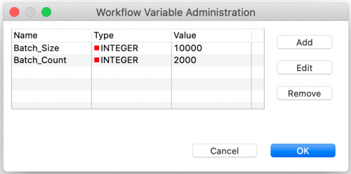
For this blog, we are going to bake 2,000 batches with each batch consisting 10,000 points for a total of 20 million sample points. Based on my empirical experimentation, this is enough samples to come to a reasonable result but without working my laptop’s processor so hard that it could bake an actual pie. To make these numbers easy to change, we will configure these settings as workflow variables:

Now that we have our recipe’s parameters set, we will start with the outer loop which controls the number of batches that we are going to cook. The Counting Loop Start node for this batch loop is configured by binding its total number of iterations to the Batch_Count flow variable.

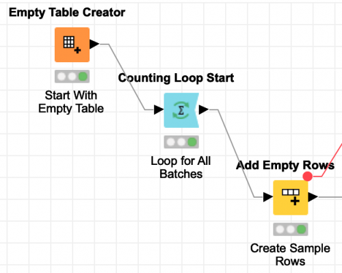
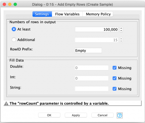
For the inner loop, we are not actually going to use a loop node in Knime. Instead, we are going to use the Add Empty Rows node to create a table with number of rows equal to the number of the sample points we want to work with in each batch. We do this using the Batch_Size flow variable to control how many rows are created in the table.

While it may be more efficient to just iterate over each point individually, capturing the set of sample points in a table allows us to visualize the sample data (such as we did for the plot of an Approximate Pi example at the start of this article). It also allows us to perform secondary analysis to help with validating our recipe as we are baking. For example, during the development of this workflow I temporarily added nodes to reassure myself that the sample point generation was reasonably pseudo-random and not falling into a cyclical pattern that would have resulted in a failure to converge on an accurate approximation. (In other words, I just wanted to prove that I didn’t screw something up for random reasons I’ll get to shortly.)

This is the beauty of KNIME – it is extremely flexible, and you can dynamically work with results as you develop your workflows. You can make trade-offs for efficiency versus ease of validation knowing that you will not be stuck on the initial path you chose. Based on my experience, I prefer to just make things work correctly first. And then I go back to optimize in order to make them work more efficiently – but I only do so if it is necessary. In this case, I don’t bake an Approximate Pi that often so I’m not particularly worried about how long it takes to bake but I do want it to come out right on the first try!

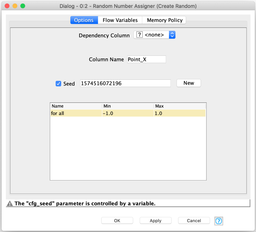
Now that we have our 10,000 empty rows of data in our current batch, we need to fill them with random sample points. Fortunately, KNIME has the Random Number Assigner node which is designed to assign a random number in a configurable range to each row in a table. We just need to do this twice for each row – once for an X coordinate and once for a Y coordinate for the sample. Simple, right?

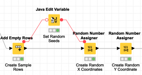
Well, not quite: working with random numbers often carries risks with it. One such risk is repeatability – if the data each run is random it is hard to reproduce issues while debugging. To mitigate this risk most random number generators allow you to specify a seed value which is used to base the pseudo-random sequence on so that each time the generator is used, it will produce the same sequence. We just need to set a seed in each of the two Random Number Assigner nodes. And of course, we wouldn’t want to use the same seed in both generators because they would then generate the same sequence for each component of the coordinates and all of our points would fall on a straight line! So different seed values it is.

But there is another more subtle gotcha lurking here. Remember that we are in a loop for each batch? If we use the same seed from batch to batch, the random sequences used in each batch will be identical and each batch will consist of the exact same set of sample coordinates. If we did not catch this bug, there will be no statistical improvement to our estimate from running multiple batches. Fortunately, this would show up in our visualization of the final results (not that I’m saying it did the first time I tried to bake with this recipe but…)

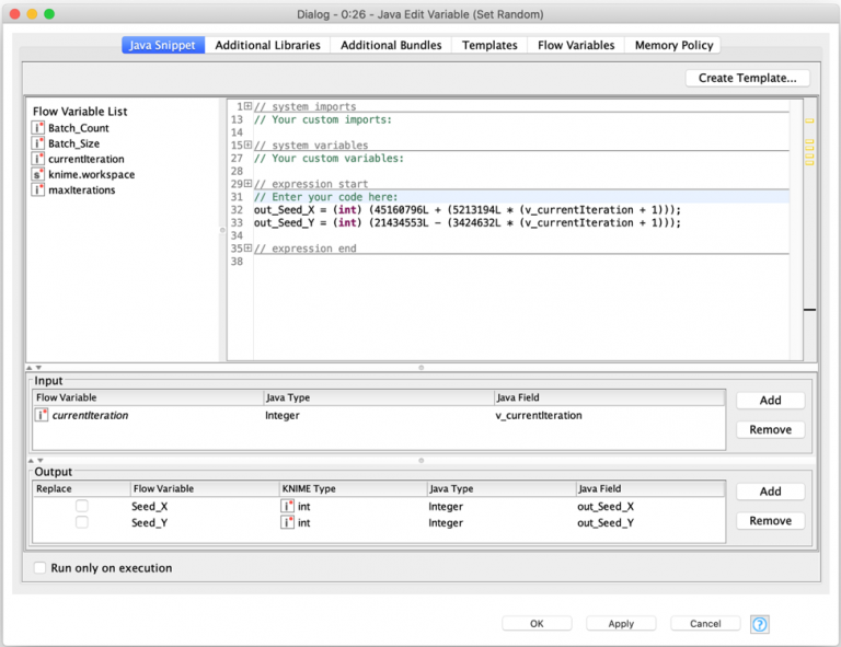
This is why our workflow contains a Java Edit Variable node to deterministically create different seed values for each Random Number Assigner. I did this with a formula based on the current iteration number so that the seeds vary for each batch but will be the same from run to run of the workflow. This results in a workflow that is repeatable; it will generate the same results each run and the results for each individual batch will be unique but the same from run to run as well.

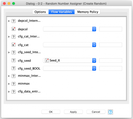
Each batch’s seed values are set as flow variables and then used by the Random Number Assigner nodes as follows:

Furthermore, each Random Number Assigner node is configured to create a coordinate column with a random value between -1.0 and 1.0. By using this range, we are assuming a circle of radius 1.0 centered at the origin. This helps simplify our calculations since area of this circle is simply the value pi.

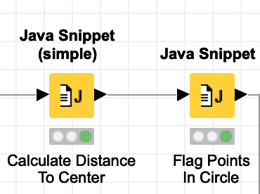
With our set of sample points generated, we now just need to figure out which ones fall inside the circle and marking those that do so that we can count them.

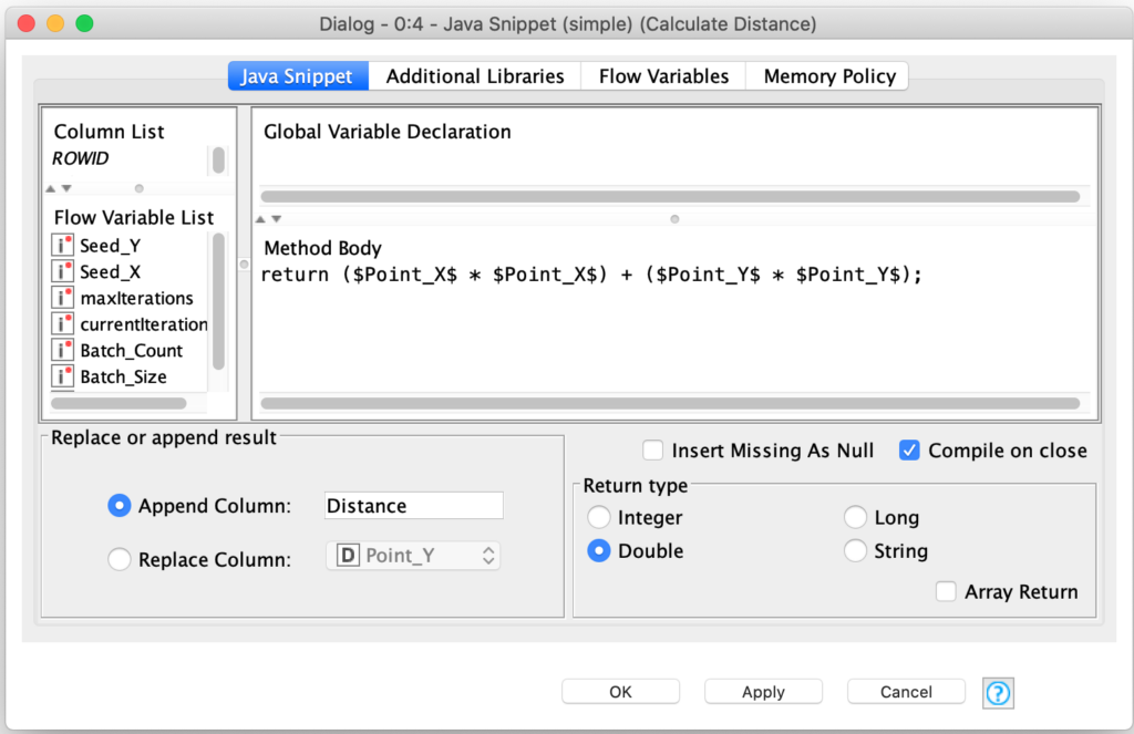
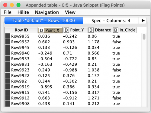
The distance calculation is simple since the circle’s center is at the origin (0,0) on the coordinate system. Furthermore, since the radius of the circle is 1.0, we do not even need to consider the square root of the distance since we are just classifying points based on whether or not they are more than 1.0 units from the origin. Since the square root of 1.0 is also 1.0, the squared distance measurement is all we need for our classification. This leaves us with the following distance calculation:

And then we immediately flag the points based on their distance value by setting a Boolean column value as follows:

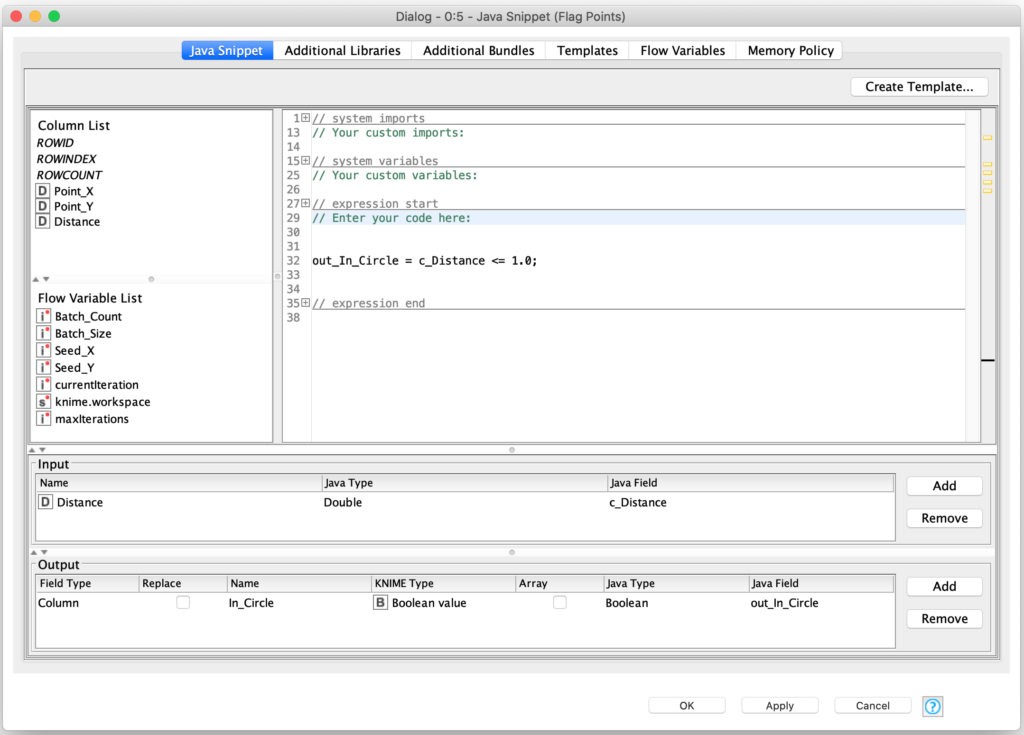
This gives us a list of labeled sample points from which we can count the number of them that have been classified as being in the Approximate Pi (circle). We can also display the points in a scatter plot to visually verify that our classification logic was correct (again, see the scatter plot at the start of this article).

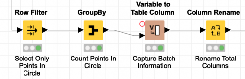
The final bit of processing in the individual batch loop is to count the number of points that were within the circle and store those alongside the total number of points in the batch. We do this with a Row Filter node to discard any points not in the circle and then a Group By node to count the remaining points. The Batch_Size flow variable is then added as a column to the result with a Variable To Table Column node and the column names are tidied up with a Column Rename node.

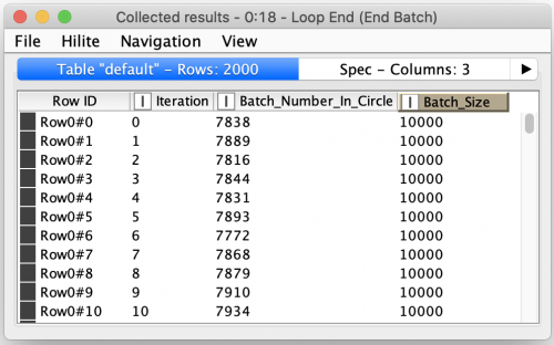
This completes the processing for each batch and the Loop End node then collects the results of all of the individual batches into one result table:

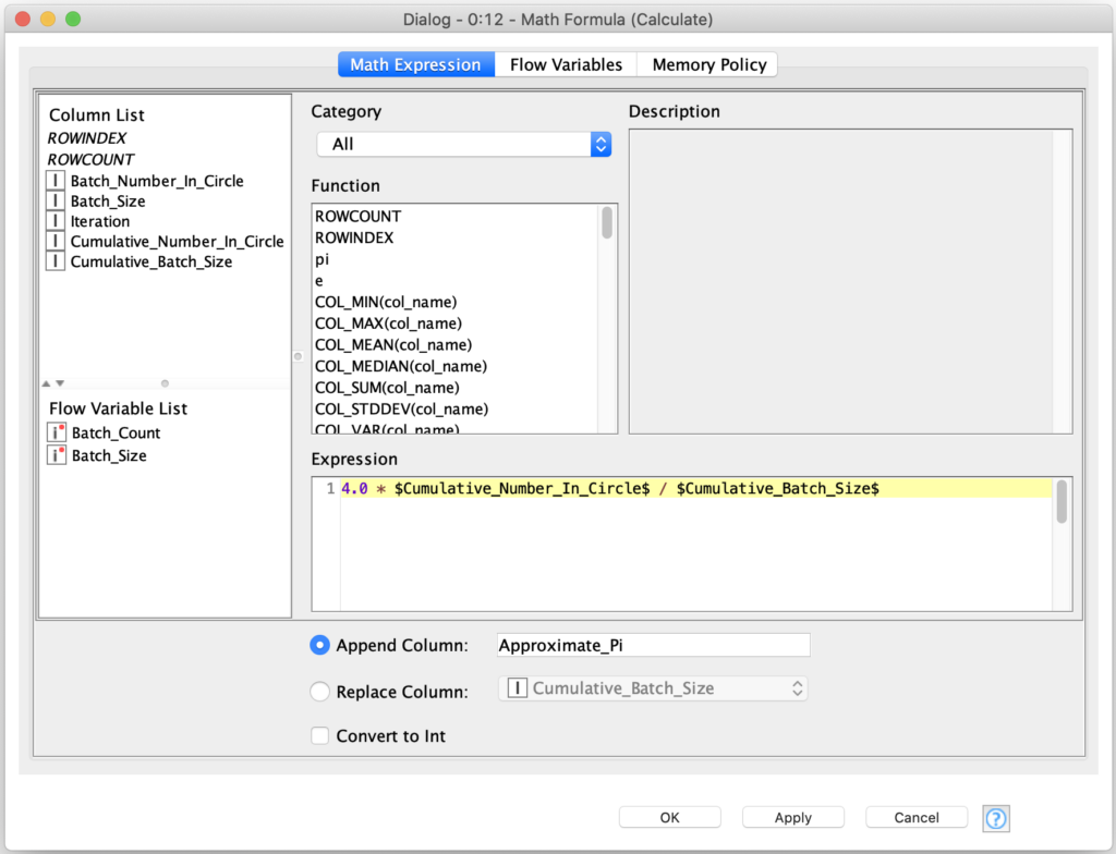
The final step of the estimation is to derive the approximate value of pi from the individual batch results. To do this we could just compute an estimate for each batch and then average them together. However, this would not allow us to visualize the convergence of the estimate over time. To show the converging estimate, we need to use running totals in our estimate’s calculation. Of course, KNIME has a node for that! We can use the Moving Aggregation node to produce these running totals:

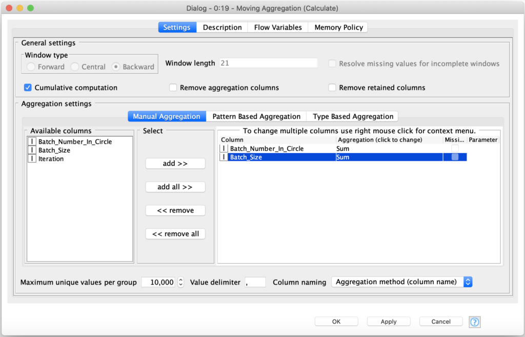
By checking the Cumulative computation option, the node will produce running totals for our two configured fields across the whole data table. We can then determine our approximated value using these running totals as well as add a column containing the actual value of pi to enhance the visualization of our results.

Computing the approximation value is straight forward, but we do need to remember that we are computing the ratio to the area of a square which was 2.0 units long on each side, for a total area of 4.0:

With the math out of the way, all that is left is to use a Line Plot and we can indeed see that our Monte Carlo recipe did a decent job of baking an Approximate Pi!

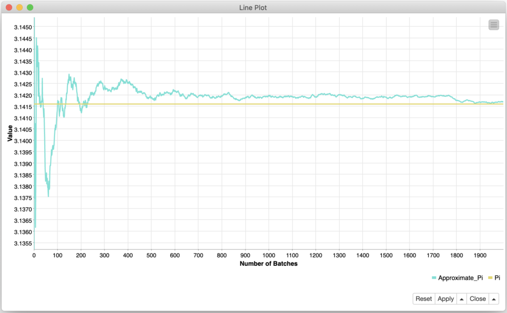
While this was a tongue-in-cheek post about solving a problem we don’t really have, it does highlight the power of computation techniques such as Monte Carlo modeling that KNIME makes ever so easy to bring to bear on real world problems. And it was tangentially about pie, which is never a bad thing even if my desire for it is irrational…