Spark: Beginner Tips & Tricks
I recently worked on a hackathon team at my company. The purpose of the hackathon was to show how to use data science on Automated Identification System (AIS) ship data to determine anchorage insights. I decided to use this hackathon as a means to learn Spark (and PySpark specifically.) My part of the project mainly involved data wrangling, to format the data and stage it appropriately for the data science operations. This document is intended to convey the key things I learned as a Spark beginner.
NOTE: All examples in this document are PySpark/Python code.
The Environment
- AWS EMR cluster
- Jupyter Notebook
- S3 storage for holding the AIS records and staged data
- Python 3
- PySpark
Lazy Evaluation
One other thing to note before we go forward. Spark code does not get executed when a line of code runs. Your code is queued up but doesn’t execute until the code is needed to perform a task. This queuing of code is called ‘Lazy Evaluation.’ For instance, if you execute a line of code to read a file, the file is not read until that data is needed somewhere else. Understanding that code in Spark is not executed immediately is important to understand because it can make development and debugging tricky if this concept Is not fully recognized.
Spark Configuration
We were dealing with a year of AIS data, which is a large dataset, which included approximately 60-90 million records per month.
While processing and analyzing the AIS data, I would occasionally run into memory errors and MaxResultSize errors on the cluster. To resolve these issues, I had to modify the cluster configuration and increase the Spark memory size.
This is done by adjusting the maximizeResourceAllocation configuration on an EMR cluster tells Spark to use all of the resources available (cores, memory, etc.) to process the job. An AWS architect may not want to use this setting in a production environment, but for my purposes, it got the job done.
To configure this setting go to the “Software Configuration” page (shown in Figure 1) of the cluster configuration.
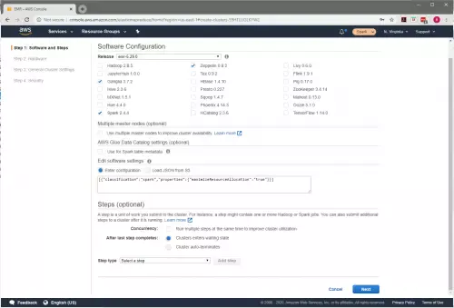
Figure 1: Software Configuration Page
Add the following configuration in the “Edit software settings” box (Figure 2: Edit software settings).
| [{“Classification”: “spark”,
“Properties”: { “maximizeResourceAllocation”: “true” } }] |
Figure 2: Edit software settings
The second configuration that I added was the maxResultSize configuration. This configuration can be set directly in your notebook. I used 4 gigabytes in this setting, but your mileage may vary. The required setting of this configuration will be dependent on your dataset. To configure this setting run the command shown in Figure 3 in a notebook cell.
| sc._conf.set(‘spark.driver.maxResultSize’, ‘4g’) |
Figure 3: maxResultSize Configuration
Dynamically Install Libraries
Prior to AWS EMR 5.26.0, in order to use an imported library in your notebook, you would need to configure that library in your cluster configuration. As of EMR 5.26.0, AWS allows notebook scoped libraries. See the documentation here:
https://docs.aws.amazon.com/emr/latest/ManagementGuide/emr-managed-notebooks-scoped-libraries.html
With notebook scoped libraries, you can quickly import required libraries for use in your notebook without having to stop and start your cluster. Figure 4 shows how to import libraries directly in your notebook dynamically.
| # SPECIAL INSTALLSsc.install_pypi_package(“pyproj”)
sc.install_pypi_package(“matplotlib”) sc.install_pypi_package(“utm”) sc.install_pypi_package(“pandas”) |
Figure 4: Notebook Scoped Libraries
UDF Functions
PySpark user-defined functions (UDF) allow a developer to use Python native code to process PySpark DataFrames and columns. There are situations where native python functions cannot process DataFrames columns. To resolve this and allow the use of native python functions on PySpark columns, we need to use UDF functions.
Implementation of UDF functions requires two steps.
- Write the python function
- Register the python function as a UDF function
Figure 5 shows how to create and register a UDF function for use in your notebook. A haversine function is a method for calculating the distance between 2 geographic points. The haversine function is a native Python function. The udf_haversine function shows how to wrap a Python function as a UDF function.
| import mathfrom pyspark.sql.functions import *
def haversine(coord1, coord2): R = 6372800 # Earth radius in meters lat1, lon1 = coord1 lat2, lon2 = coord2 phi1, phi2 = math.radians(lat1), math.radians(lat2) dphi = math.radians(lat2 – lat1) dlambda = math.radians(lon2 – lon1) a = math.sin(dphi/2)**2 + math.cos(phi1)*math.cos(phi2)*math.sin(dlambda/2)**2 return 2*R*math.atan2(math.sqrt(a), math.sqrt(1 – a)) # Package the distance method as udf udf_haversine = udf(lambda lat1, lon1, lat2, lon2: haversine((lat1, lon1), (lat2, lon2)) / 1000, returnType=FloatType()) #Define UDF function |
Figure 5: Spark UDF Functions
The code in Figure 6 shows how to call the UDF function from your code. The columns lat_lag1 and lon_lag1 refer to the location from the previous AIS record, and lat and lon refer to the location from the current AIS record.
| # CALCULATE DISTANCE BETWEEN 2 LOCATIONSdf = df.withColumn(‘distance_lag1’, udf_haversine(df.lat_lag1, df.lon_lag1, df.lat, df.lon)) |
Figure 6: Call a UDF Function
Reading a Parquet File from an S3 Bucket
Reading a file from an S3 bucket is a straightforward but essential task for processing data. Figure 7 shows how to read a parquet file from an S3 bucket. Notice that I first set up an array of StructField objects to define the schema. The array allows me to specify the datatypes for the resulting DataFrame.
- createDataFrame creates an empty DataFrame
- read.load reads the file and loads it into the DataFrame
| from pyspark.sql.types import *from pyspark.sql import SQLContext
from pyspark.sql.functions import * field = [StructField(‘mmsi’,StringType( ), True), StructField(‘lat’,FloatType( ),True), StructField(‘lon’,FloatType( ),True), StructField(‘course’,FloatType( ), True), StructField(‘heading’,FloatType( ), True), StructField(‘speed’,FloatType( ), True), StructField(‘maneuver’,IntegerType( ), True), StructField(‘radio’,IntegerType( ), True), StructField(‘repeat’,IntegerType( ), True), StructField(‘seconds’,IntegerType( ), True), StructField(‘status’,IntegerType( ), True), StructField(‘turn’,IntegerType( ), True), StructField(‘imo’,StringType( ), True), StructField(‘callsign’,StringType( ), True), StructField(‘shipname’,StringType( ), True), StructField(‘shiptype’,StringType( ), True), StructField(‘destination’,StringType( ), True), StructField(‘eta’,TimestampType( ), True), StructField(‘draught’,StringType( ), True), StructField(‘distancetobow’,FloatType( ), True), StructField(‘distancetoport’,FloatType( ), True), StructField(‘distancetostarboard’,FloatType( ), True), StructField(‘distancetostern’,FloatType( ), True), StructField(‘timereceived’,TimestampType( ), True)] schema = StructType(field) parquetFile = sqlContext.createDataFrame(sc.emptyRDD(), schema) parquetFile = spark.read.load(“s3://grc-ais/stage0/datereceived=2015-02-*”) |
Figure 7: Reading from a Parquet File
Writing a Parquet File to an S3 Bucket
To perform tasks in parallel, Spark uses partitions. For a file write, this means breaking up the write into multiple files. The multiple files allow the write to execute more quickly for large datasets since Spark can perform the write in parallel.
Figure 8 shows how to define a partition for a file. In this case, I used the date of the record to determine which file to place the record. It also shows how to write the file using partitions.
| # WRITE THE DATAFRAME RECORDS TO A PARQUET FILEdf = df.withColumn(‘track_datereceived_end’, df.track_timereceived_end.cast(“date”))
df.write.partitionBy(“track_datereceived_end”).mode(‘overwrite’).parquet(‘s3://XXXXXX/stage1/’) |
Figure 8: Write Parquet File
How to use Windowing on a DataFrame
Windowing on a DataFrame is similar to windowing in SQL; it allows you to view other records in the DataFrame beyond the current record. There are many things you can do with windowing; this will be a cursory overview.
When you are processing a DataFrame, you process each record in the DataFrame similar to the way a SQL statement would process each record in a database table. For instance, take the code in Figure 9
| df.withColumn(‘new_column’, df.colA + df.colB) |
Figure 9: withColumn Example Code
This code adds a new column that is the sum of colA and colB of the current record that is being processed. But what if we wanted to sum colA from the previous record in the set with the current record in the set. ColA from the previous record is not available to us under normal circumstances. This need to see the previous record is where ‘windowing’ comes in. It allows us to peer into other records within the dataset while processing the current record.
Here is an article with an in-depth look at Windowing on DataFrames.
https://databricks.com/blog/2015/07/15/introducing-window-functions-in-spark-sql.html (Editor’s note 4/13/26: article no longer available)
Using DataFrame windowing requires two steps:
- Configure the window
- Use the window to view records outside the current record
The first example shown in Figure 10 shows how to window to the previous record. The first step is to configure the window (here it is assigned to a variable ‘w’). Notice that the window has a ‘partitionBy’ and an ‘orderBy.’ An ‘orderBy’ is required to use the ‘lag’ function.
Then we use the ‘lag’ function to pull the ‘lat,’ ‘lon,’ and ‘timereceived’ from the previous record onto the current record.
| from pyspark.sql.functions import *from pyspark.sql.window import Window
w = Window().partitionBy(“mmsi”).orderBy(col(“mmsi”),col(“timereceived”)) parquetPlus = parquetClean.select(“*”, lag(“lat”).over(w).alias(“lat_lag1”), lag(“lon”).over(w).alias(“lon_lag1”), lag(“timereceived”).over(w).alias(“timereceived_lag1”)) |
Figure 10: Windowing to the Previous Record
With DataFrame windowing in addition to the ‘lag’ function, you can also use ‘first’ to get the first record in the partition, ‘last’, to get the last record in the partition. Furthermore, you can use aggregation functions such as count, sum, average over a Windowing partition.
Matplotlib Visualizations in Spark
Visualizing the data for analysis is an important part of data science. Using matplotlib we can visualize our data using graphs like line chart, bar charts, or scatter graphs.
Though visualizing data using matplotlib in Pandas is a common task, doing this with PySpark in an EMR notebook took me a while to figure out, so I will be listing several tips in this section that are important to make this work.
Figure 11 shows the code I used to visualize my data for analysis. I will breakdown this code for you.
- Remember, I had previously imported the matplotlib library as a notebook scoped library.
- Notice the imports: I imported the entire matplotlib library and have a second import for pyplot from that library
- I assigned my DataFrame to a variable called df_plot
- I bucketed my DataFrame data suitable for a bar chart according to the buckets
- I used a groupBy function to facilitate the aggregation
- I converted my Spark DataFrame to a Pandas DataFrame
- I executed the plot function, configured as a bar graph to display the buckets in the visualization
| from pyspark.sql.functions import *import matplotlib
import matplotlib.pyplot as plt # testColumn = ‘track_distance_km’ # testColumn = ‘track_segment_duration_hours’ testColumn = ‘p_cluster_distance_km’ df_plot = dfProcessedRecords df_plot = df_plot.withColumn(“test_bucket”, when(col(testColumn) > 10000.0, 10001)) df_plot = df_plot.withColumn(“test_bucket”, when(col(testColumn) < 10000.0, 10000).otherwise(col(“test_bucket”))) df_plot = df_plot.withColumn(“test_bucket”, when(col(testColumn) < 7500.0, 7500).otherwise(col(“test_bucket”))) df_plot = df_plot.withColumn(“test_bucket”, when(col(testColumn) < 5000.0, 5000).otherwise(col(“test_bucket”))) df_plot = df_plot.withColumn(“test_bucket”, when(col(testColumn) < 2500.0, 2500).otherwise(col(“test_bucket”))) df_plot = df_plot.withColumn(“test_bucket”, when(col(testColumn) < 1000.0, 1000).otherwise(col(“test_bucket”))) df_plot = df_plot.withColumn(“test_bucket”, when(col(testColumn) < 500.0, 500).otherwise(col(“test_bucket”))) df_plot = df_plot.withColumn(“test_bucket”, when(col(testColumn) < 100.0, 100).otherwise(col(“test_bucket”))) df_plot = df_plot.withColumn(“test_bucket”, when(col(testColumn) < 75.0, 75).otherwise(col(“test_bucket”))) df_plot = df_plot.withColumn(“test_bucket”, when(col(testColumn) < 50.0, 50).otherwise(col(“test_bucket”))) df_plot = df_plot.withColumn(“test_bucket”, when(col(testColumn) < 25.0, 25).otherwise(col(“test_bucket”))) df_plot = df_plot.withColumn(“test_bucket”, when(col(testColumn) < 10.0, 10).otherwise(col(“test_bucket”))) df_plot = df_plot.withColumn(“test_bucket”, when(col(testColumn) < 2.0, 2).otherwise(col(“test_bucket”))) df_plot = df_plot.withColumn(“test_bucket”, when(col(testColumn) < 1.0, 1).otherwise(col(“test_bucket”))) df_plot = df_plot.groupBy(“test_bucket”).count().orderBy(‘test_bucket’, ascending=True) df_plot = df_plot.toPandas() df_plot.plot(kind=’bar’, x=’test_bucket’,y=’count’, rot=70, color=’#bc5090′, legend=None, figsize=(8,6)) |
Figure 11: Charting using MATPLOTLIB
Now, because of ‘Lazy Evaluation’ nothing happens yet. To display the plot EMR notebooks include a ‘magic’ function that executes the previous code. This ‘magic’ function is shown in Figure 12. Execute this code to display your chart in the notebook.
| %matplot plt |
Figure 12: matplotlib magic function
The key to making this visualization work is that I needed to convert my DataFrame to a Pandas DataFrame. However, Pandas is not very good at dealing with Big Data, so make sure that you aggregate your data appropriately before you convert your DataFrame.
Also, I needed to execute the ‘magic’ function in a separate cell; otherwise, I received errors.
Conclusion
These are just a few of the most important things I learned as I worked my way through my initial effort with Spark. I hope these tips were useful for you. I was able to process 10s of millions of records in a relatively short period of time. Spark is a powerful tool that makes quick work of Big Data.